Elliptic Curves In-Depth (Part 1)

Cryptography is always evolving.

New techniques are being developed all the time. Especially in some fields that seem to be all the rage nowadays, such as Zero-Knowledge proofs, Fully Homomorphic Encryption, and Post-Quantum Cryptography.

Better, faster, more secure methods are constantly being researched. The sheer amount of cryptographic techniques out there is overwhelming.

However, the fundamental mathematical structures upon which this world of diverse techniques is based is rather invariant.

Although there are perhaps some new faces on the block like polynomial rings and ideals, and some research on more exotic alternatives like p-adic numbers.

Most of the cryptographic methods we use every day (often times without even noticing) are based on a single construction: an elliptic curve.

It’s possible that they become obsolete soon. But at least in the very near future, they are going nowhere!

I recently talked about them in the Cryptography 101 series. Truth be told, that was only a brief, friendly overview of the topic. Good enough as a first approach — but not nearly close to the full story.

This time around, I want to take a stab at a deeper dive into the world of elliptic curves. There’s a lot to cover, so I’ll be splitting this into a few parts.

Hope you enjoy!

Elliptic Curves

Naturally, the first question that comes to mind is what the hell is an elliptic curve?

Without much further ado, I present to you — this is an elliptic curve:

$$E: y^2 + a_1xy + a_2y = x^3 + a_3x^2 + a_4x + a_5$$

What you’re looking at is the general Weierstrass equation for elliptic curves — it’s really just a cubic (degree three) polynomial. Nothing to be scared of.

In general, we’ll use the following reduced version, which is equivalent under some conditions that we’ll not cover here:

$$E: y^2 = x^3 + ax + b$$

And this is what an elliptic curve looks like when plotted in a cartesian plane:

Click to zoom

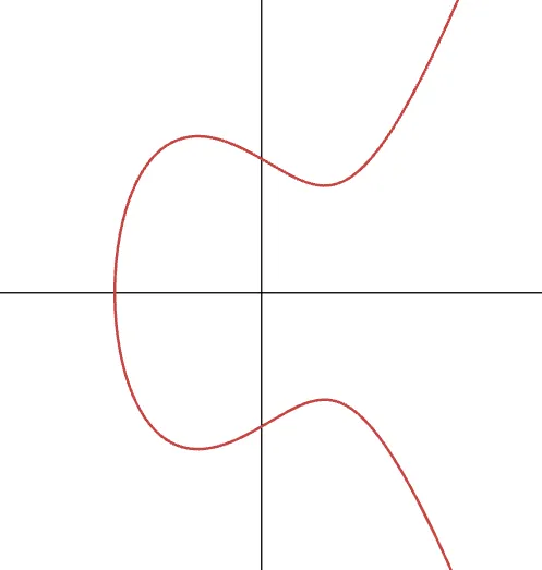
Looking at this figure, you may wonder what’s “elliptic” about these curves. It just so happens that this is somewhat of a misnomer, as explained here.

What we’re representing here is the collection of points that satisfy the equation $E$ we defined previously, just like a parabola satisfies the equation $y = x^2$.

Now, there are a couple things we can say about these curves from the get go.

First off, notice how they are symmetric about the x-axis. It’s easy to see that the culprit is that $y^2$ term, because any positive value for $x^3 + ax+ b$ has both a positive and a negative square root, which are both valid solutions for $y$.

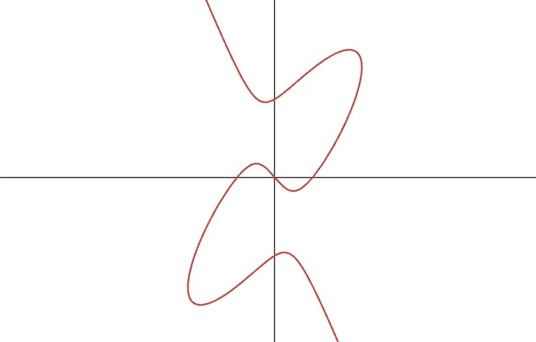
Secondly, the curve is smooth. Not all curves that satisfy the expression $E$ are smooth, though — like this one:

Click to zoom

We can see how there seems to be an intersection point. If you try plotting the curve $y^2 = x^3$, you’ll also notice some strange behavior.

It’s technically not an intersection, but rather two pointy parts of the curve touching each other.

We call these kind of curves singular. Singular curves will be problematic when we try to use them for our intents and purposes — because the derivative at those points isn’t well-defined. For this reason, non-smooth curves such as this one are not considered to be elliptic curves.

So much for presentations! What are these little thingies good for anyway?

Defining Operations

What’s attractive about these curves is that we can use them to define an operation. I want to dedicate the remainder of this article to understanding said operation, which leaves its usefulness out of the picture for now — but we’ll cover that in coming articles.

Still, I’d like to provide some context before moving on.

Our operation will serve as a key piece in the construction of a mathematical group. We’ll talk about those later — but the idea is that groups are the cornerstone for some crazy hard math problems, that enable the public key cryptography we all know and love. And then some.

The elliptic curve operation we’re going to present has sort of a weird definition. Please bear with me for now. It goes like this:

1. Pick two points $P$ and $Q$ on the curve, and draw a line through them.
2. You’ll find that this line intersects another point on the curve. Let’s call it $-R$.
3. Now, flip $-R$ about the x-axis. Since $-R$ is a point on the curve, and the curve is symmetric, you’ll arrive at another point on the curve: $R$.

The whole process looks something like this:

Click to zoom

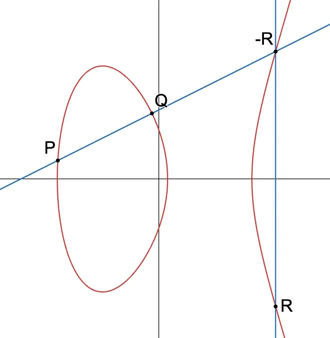
By following this recipe, we’ve calculated a new point $R$ as the result of “adding” $P$ and $Q$. We can write this as:

$$P \oplus Q = R$$

It’s a strange way to define addition, yes — but it’s helpful to think about the operation in those terms. We use the symbol $\oplus$ to differentiate it from “normal” addition.

What happens if we want to add $P$ to itself, though?

Imagine, instead, that we have some other point that’s really close to $P$ on the curve — let’s call it $P’$. As we move $P’$ closer and closer to $P$, the line going through them slowly approaches the tangent of the curve at $P$. Very naturally, we can infer that finding $P \oplus P$ is done with the same process from before, but using the tangent at $P$ as our line in the first step.

And this is why having a well-defined first derivative is important!

To the surprise of absolutely nobody, the recipe we followed is called the chord-and-tangent rule. Does it always work, though? Aren’t there any border scenarios that may be troublesome?

The Point of Intersection

In step one of our chord-and-tangent rule, one important assumption is that we can find a third intersection point. Is this always possible? Let’s take a closer look — time for some substitutions!

The equation for a line $l$ is very simple:

$$l: y = mx + n$$

What’s nice is that we can substitute this expression directly into our elliptic curve equation, yielding this third-degree polynomial equality in $x$:

$$(mx + n)^2 - x^3 - ax - b = 0$$

A third-degree polynomial such as this one has at most three roots. And as you might guess, those roots will be the x-coordinates of the points where our line intersects the curve, if there happens to be any intersection at all.

Let’s try and figure out happens when we use this expression in the cases of the chord-and-tangent rule.

The Chord

If our polynomial has three roots, then we can factorize it into a product of terms of the form $(x - r)$. And with some rearranging, we end up with:

$$(x - x_P)(x - x_Q)(x - x_R) = x^3 - m^2x^2 + (a - 2mn)x + b - n^2$$

We've not yet figured out what the values for $m$ and $n$ are - but they are pretty easy to calculate for a line going through two points (P and Q), so I'll leave that part to you.

It's useful to expand the left-hand side of the expression above, which yields:

$$x^3 - (x_P + x_Q + x_R)x^2 + (x_Px_Q + x_Px_QR + x_Qx_R)x - x_Px_Qx_R$$

And look at this: comparing the $x^2$ term on both sides of the equation, we get:

$$x_P + x_Q + x_R = m^2$$

By moving a couple terms to the right, we've obtained an expression for the x-coordinate of this third point of intersection. To find $y$, all we have to do is plug it into the line equation, and then flip the resulting value. And we're left with:

$$x_R = m^2 - x_P - x_Q$$ $$y_R = -(mx_R + n)$$

That's all!

The Tangent

Finding $R$ is a little trickier now, because we need to find the line going through $P$ that's tangent to the curve. The tangent is simply the line that goes through $P$ whose slope is equal to the first derivative of the curve with respect to $x$.

Since we don't have an explicit formula in the form of $E(x)$, we have to dust off our calculus skills, and use a little old trick called the chain rule, by treating $E(x)$ as an implicit function:

$$\frac{d}{dx}(y^2) = \frac{d}{dx}(x^3 + ax + b)$$ $$\frac{dy^2}{dy}\frac{dy}{dx} = 3x^2 + a$$ $$\frac{dy}{dx} = \frac{3x^2 + a}{2y^2}$$

Upon plugging the coordinates of $P$ into the above expression, we find the slope of the line tangent to $E$ in $P$ - this was our value $m$ in the previous case.

$$m = \frac{3x_P^2 + a}{2y_P^2}$$

Then, we proceed as before. We just need to be careful to consider $x_P$ a root with multiplicity = 2. With this in mind, we get almost exactly the same result:

$$x_R = m^2 - 2x_P$$ $$y_R = -(mx_R + n)$$

Adding $P$ to itself is like doubling it. And so, instead of writing $P \oplus P$, let's write $[2]P$, and we refer to this as - you guessed it - point doubling!

An Edge Case

Cool! Everything working nicely so far.

Now we could try adding $P$ and $-P$ (its reflection over the x-axis). However, the line passing through them is a vertical line, defined by $x = x_P$. This means that we'll get:

$$y_P^2 = x_P^3 + ax_P + b$$

For a given $x_P$ value, this means that we get two valid values for $y_P$, not three. Not good - step 1 of our process requires a third point of intersection to exist. Or does it?

Clearly, for our operation to be well defined, we need to be able to perform $P \oplus (-P)$. If this was a simple addition, this would of course result in zero. Essentially, what we need is to define what zero means for our operation.

Well, here it is: I present to you the point at infinity:

$$P \oplus (-P) = \mathcal{O}$$

Click to zoom

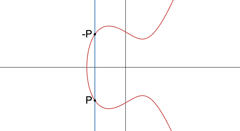
I ask you to stretch your imagination a little at this point. If anything, think of this as a "special point". Whenever we need to add $P \oplus (-P)$, we know that the normal chord rule does not apply, and instead, we know the result to be the point at infinity, $\mathcal{O}$.

We'll make some more sense out of this when we talk about projective space.

Fast Addition

Another particularly cool thing about this operation we defined is that there's an algorithm for fast addition. This is, if we wanted to add:

$$P \oplus P \oplus P \oplus ... \oplus P \oplus P = [m]P$$

We could do this one step at a time, adding $P$ to the result of each subsequent sum, as we already know how to do.

Surprisingly, we can do better. Because the operation is associative, it's possible to "batch" additions, in a way that might be convenient to us. For instance, $[5]P$ can be written as:

$$[5]P = (P \oplus P) \oplus (P \oplus P) \oplus P$$ $$= [2]P \oplus [2]P \oplus P = [2]([2]P) \oplus P$$

Observe that the final expression requires two doublings and one addition, as opposed to the four additions required in the initial setup. Saving a single operation might not seem to amount to much, but when we multiply by a larger $m$, the savings are substantial.

The general algorithm for multiplication works in a double and add fashion. For any positive integer $m$ we want to multiply by, we first need to find its binary representation, and do the following process:

1. Set the initial value of the result to $W = P$.
2. Then, starting from the second most significant bit, assign $W = [2]W$.
3. If the current digit is a $1$, then also add $W = W \oplus P$.
4. Move one digit to the right, and repeat from step $2$.

For example, $11$ in binary is $1011$. The process would have 3 iterations total:

• Initialization: $W = P$
• First digit: $W = [2]W = [2]P$
• Second digit: $W = [2]W \oplus P = [5]P$
• Last digit: $W = [2]W \oplus P = [11]P$

A grand total of $3$ multiplications and $2$ additions - already half of the $10$ additions necessary if we added one $P$ at a time.

Typically, this is called multiplication by $m$ instead of "fast addition". We do have a fast algorithm though - and importantly, the inverse problem is not fast at all.

By this, I mean that given two points $G$ and $Q$, such that $Q = [m]G$, there's no fast algorithm to work back the value of $m$.

Such a simple is what enables a good deal of the public key cryptography we know and love!

But Why Elliptic Curves?

Oh boy. Already with the spicy questions.

We still don't really know a lot about how elliptic curves are useful from a cryptographic perspective. All we know is how to add points together, following a process that, given our current knowledge, looks very arbitrary and quite honestly, a bit forced.

Of course, lots of things remain to be said about elliptic curves - but we can at least try and imagine a couple things.

There's a theorem called Bézout's theorem that, loosely speaking, says that a line will intercept a degree-three curve in 3 points (counting the point at infinity and stuff). Our operation is then fairly natural - given two points in the curve, drawing a line through them guarantees we'll find a third, and this is useful to get a unique result.

What if we tried to use a higher-degree curve? Because of Bézout’s theorem, we have more than just 3 intersection points. Which means, if we want to add two points $P$ and $Q$ on the curve, we’ll have multiple candidates as our result. Which one do we choose?

Click to zoom

This makes defining an operation over these types of curves kinda complicated.

It’s possible, using a concept called divisors. But it’s still far too early to talk about that.

If we somehow had a way to define an operation over higher-degree curves, the other problem we’d have is impracticality. Finding expressions for the intersection points was simple with our trusty elliptic curves, but it can be a mess with more complex curves. Explicit formulas may not even be available, due to the Abel-Ruffini theorem.

We said we’d work with the Weierstrass form, but this doesn’t mean that there aren’t other degree-three curves we could use. For instance, there are the Mongomery curves and Edwards curves, which are also useful for cryptography, but they are perhaps not the ones with the most widespread adoption.

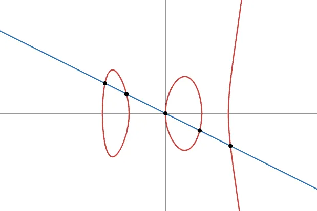
Also, we could think of slightly more complex degree-three curves, such as this one:

Click to zoom

Try as you may, you’ll find that a line intersects this curve at most at three points. But this doesn’t mean it’s very practical to use — in fact, explicit formulas will not be easy to derive, and will probably be more computationally complex than our simple Weierstrass results.

In this sense, our elliptic curve definition sits in sort of a “goldilocks” zone, balancing low computational costs of operations, while providing enough complexity to be useful in cryptography.

And about those explicit formulas I keep mentioning, we’re one hundred percent going to need them if we want to build any algorithms out of our curves. You see, these visualizations are great as a way to build up an initial understanding, but fail to represent how an elliptic curve will really look like to us, which more closely resembles this:

Click to zoom

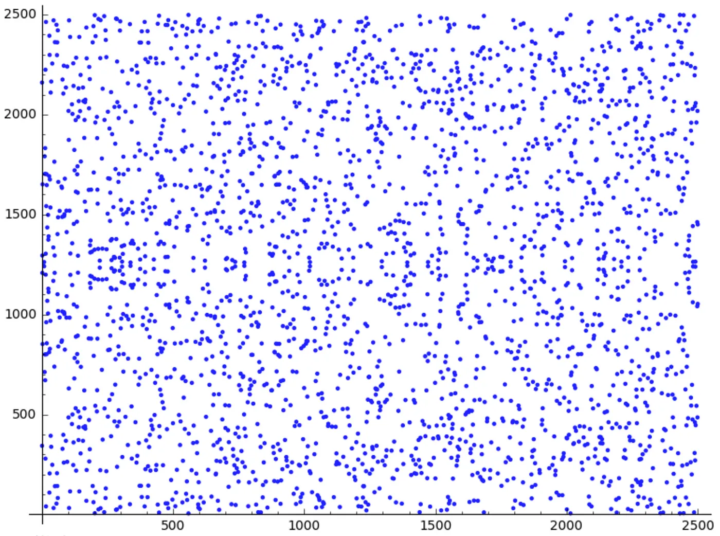
I get the feeling you probably just went:

Don’t worry — it will all make sense soon!

Summary

In this first part of what will (hopefully) be a short series of articles, we presented the basics about elliptic curves.

If you already read this, or if you had prior knowledge of the subject, you’ll probably find this introduction very simple.

But we’re just getting started! We’ve got a lot of fun stuff to cover — from million-dollar problems, to curves on “higher dimensions”.

Stay tuned, and I’ll see you on the next one!