Cryptography 101: Post Quantum Cryptography

This is part of a larger series of articles about cryptography. If this is the first article you come across, I strongly recommend starting from the beginning of the series.

Now that the basic theory around the ring learning with errors problem and ideal lattices is covered, the next natural step is to put them to good use.

In 2016, the US National Institute of Standards and Technology launched an initiative called the Post-Quantum Cryptography Standardization Project. The idea was to receive nominations for quantum-resistant algorithms (more on this in a moment) in the hopes of selecting the best candidates and standardizing a set of techniques that could be used to build the next generation of a secure web.

After a few years, four winners were announced — and three of them were lattice-based algorithms.

In this article, we’ll look at how some of these algorithms work and also take some time to discuss how quantum computers threaten the cryptographic methods that secure our day-to-day communications.

Quantum Computing in a Nutshell

I’m not an expert in the field of quantum mechanics at all (although I’ve taken a course or two). With my limited knowledge, I can say that it’s quite a complex topic, and it’s even challenging to wrap your head around some of the most basic and foundational ideas. This is the reason why we won’t go into much detail about how quantum computers work. Still, a little primer is in order to understand why it’s important to worry about their computing power.

Our everyday computers operate using electric current, which is essentially used to represent binary numbers. You know, current flowing indicates a $1$, and current not flowing indicates a $0$ — that’s what we know as a bit. Each bit can only represent two states.

Moreover, operations in traditional computers are performed sequentially, meaning that you need to read some bits of data, perform an operation (like addition), store the resulting data… And only then are you allowed to move to the next operation.

This has worked abundantly well for humanity. Computers are capable of solving all sorts of problems really fast, which has helped develop many areas of knowledge.

And they also gave us Minecraft.

But, for some operations, these simple limitations make solving some problems absolutely infeasible. In fact, that’s what cryptography is about: creating puzzles hard enough that our current computing power cannot solve in a reasonable time.

Quantum computers are built differently. The fundamental unit of information is the quantum bit or qubit for short. A qubit can exist in a state that’s neither $0$ nor $1$. It exists in a superposition of both states, which sort of means that it’s a combination of states.

A possible analogy is a guitar string vibrating. As it vibrates, it makes a sound, so its “state” is super real to us. But how do we mathematically describe said vibration? Well, we can describe it as a combination of different “simple” vibration patterns called vibration modes.

This is what superposition essentially does: represent the current state as a pondered sum of simpler parts. They may be infinitely many parts, but that’s acceptable!

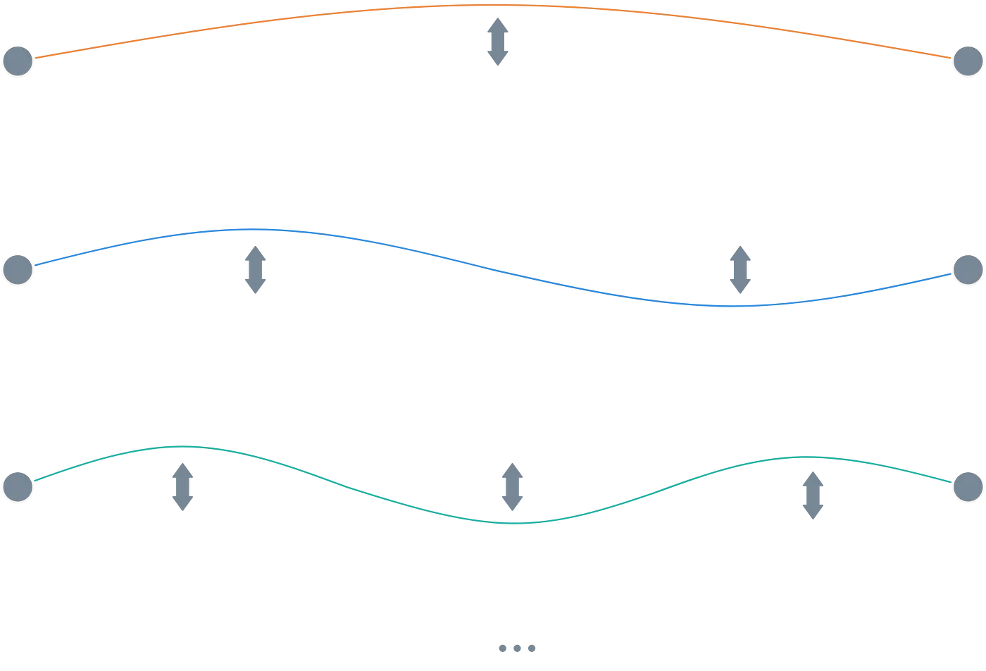
Because a qubit encodes much more information than a simple $0$ or $1$, it enables multiple operations to be executed at the same time. And this increases exponentially the more qubits we have.

The result of this (together with a couple more odd terms that we haven’t even mentioned, like wave function collapse and entanglement) is much, much faster computing. So much so that our current elliptic-curve-based methods would not stand much of a chance!

We could run Shor’s algorithm and make short work of problems such as the prime factorization problem.

Quantum computers are not very practical today — it’s unlikely you’ll be reading this article in one any time soon. But we never know what the future may hold, and even if quantum computers are not for everyday use, specialized facilities hosting them could crack complex problems really fast and break our current security models.

In sum:

Current ECC methods can be cracked with quantum computers, so we need better, more secure algorithms.

This is the main reason why PQC has been such a hot topic recently: to try and protect information from this latent threat. Lattice-based problems are thought to be so hard that not even quantum computers can solve them quickly.

With this promise of robustness and security, let’s take a look at two of the algorithms proposed by NIST for standardization. But before that...

Key Generation

Both algorithms will share the same construction for private and public keys. This is very reminiscent of elliptic curve cryptography, where the keys were almost always a big integer $d$ (private key) and a point $[d]G$ in the elliptic curve (public key).

This time around, though, the keys will involve rings and base their security on the RLWE problem we already saw in the previous article.

Okay, enough preamble! Let’s see how this works.

Much like you need to select an elliptic curve for any ECC method (like ECDSA), we’ll need to select a ring here and also some public parameters for the system.

First, we choose the ring $R$, usually of the form:

$$R = \mathbb{Z}_q[X]/(X^n + 1)$$

We’ll then sample a bunch of random polynomials from it. These will be placed in a $k \times l$ matrix we’ll call $A$:

$$A \in R^{k \times l}$$

The pair $(R, A)$ is akin to the pair $(E, G)$, where $E$ is an elliptic curve, and $G$ a generator. No surprises here!

With this at hand, key generation is quite simple. We need some secret information for our private key — these will be two vectors of polynomials, one of length $l$ and one of length $k$.

$$\\ s_1 \in R^l \\ s_2 \in R^k$$

They have a particularity, though — they are short polynomials. In this context, short relates to the vector representation of each polynomial, which, as you may recall, comes from using the coefficients as the coordinates of a vector.

For a vector to be “short,” we need the coefficients to be small. And so, to sample these $s_1$ and $s_2$ polynomials, we also require the coefficients to be small, typically limited to a range $\{−\eta, ..., \eta \}$, where $\eta$ is a small integer.

Just like error polynomials or vectors!

We have our private key $(s_1, s_2)$. With them, we just calculate:

$$t = A.s_1 + s_2 \in R^k$$

The public key will simply be$(A, t)$. Notice that recovering $s_1$ and $s_2$ from $A$ and $t$ involves solving the RLWE problem — which means we can safely share the public key!

Asymmetric keys, check. We can now move into our methods for today.

Kyber

CRYSTALS Kyber is formally a Key Encapsulation Mechanism (KEM), which means that it’s a way for a sender to transmit a short secret message over a network in a secure way — and a receiver can then recover said secret.

It’s similar to encryption but generally used for a different purpose, such as transmitting symmetric keys for later use in subsequent communications.

This technique consists of three fairly standard steps: key generation, encapsulation (similar to encryption), and decapsulation (which is analogous to decryption).

Luckily, we already know how key generation works. A receiver will generate a public key $(s_1, s_2)$ and share the associated public key $(A, t)$ with the sender of the message.

With this, we can move directly onto the second step.

Encapsulation

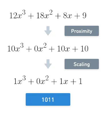
Alright, this starts pretty much like you’d expect encryption to work: a sender wants to share a value $M$ with a receiver. But what happens next may sound quite exotic to us: they transform said value into its binary representation — and then encode the digits into a polynomial. Not only that, but they then scale that polynomial by a factor of half the field size, rounded.

Yeah, that was probably a lot to take in. I think trying to visualize this will help us understand the process, so let’s continue with a toy example.

Take the number $13$. It’s binary representation is $1101$. From right to left, if we map each digit to a power of $x$, this is the polynomial we end up with:

$$x^3 + x^2 + 1$$

Then, suppose we’re working with modulo $19$. We need to scale this polynomial by a factor of half of $19$, which, rounded, results in $10$. And so, our value $13$ has been transformed into:

$$10x^3 + 10x^2 + 10$$

I know, definitely not what we’re used to — this part might be a bit of a head-scratcher, but I promise it’ll make sense in a minute.

So, we have our message in polynomial form — let’s call it $m$. What the sender needs to do now is calculate the ciphertext. For this, they sample three random vectors: $r$, $e_1$, and $e_2$, and perform these operations:

$$u = A^T.r + e_1$$ $$v = t^T.r + e_2 + m$$

The $T$ superscript means we take the transpose of a vector or matrix.

And the resulting ciphertext is just $(u, v)$. This is sent to the receiver, who proceeds to decapsulate.

Note that we can draw some parallels with ECC here: $r$ is what we usually call a nonce, and we need one value to encode the nonce ($u$) and the other one to encode the message along with the nonce ($v$).

Decapsulation

The final step is very straightforward, but it is actually where we find the secret sauce that makes all this mess work.

The receiver simply calculates:

$$m' = v - {s_1}^T.u$$

Doing the substitutions and cancelations, what the receiver gets is:

$$m' = m + {s_2}^T.r + {s_1}^T.e_1 + e_2$$

Huh... That’s weird. Normally, decryption processes yield back the original message, but that’s not the case here. What’s going on? It seems we’re in a pickle. Did we hit a dead end?

Of course not! You see, the difference between $m$ and $m’$ is just a bunch of polynomials. If they are small, then $m$ and $m’$ will be very close in value. And because we applied a suitable scaling before sending the information, then the coefficients of $m’$ will be close to either $0$ or $10$!

It helps that we chose $s_1$, $s_2$, $e_1$, and $e_2$ as small polynomials! Yay!

Thus, for each coefficient, we just pick whichever is closer — $0$ or $10$. Finally, we revert the scaling by dividing by $10$ and recover the original message!

Visually:

Click to zoom

It’s fairly complex, I know. But in essence, it’s not much different from other encryption methods: the sender has some sort of public key, performs a couple of operations, and sends some ciphertext only decodable with the receiver’s private key.

The nice thing is as the field and polynomial sizes become larger, this problem becomes unimaginably hard to solve without knowledge of the secret information. Awesome!

For more information on this method, I suggest reading this article or this other one, or watching this video:

Dilithium

Apart from encryption, we use to think of digital signatures as the other type of primitive operation in cryptography. It stands to reason that this is the next kind of algorithm we’d like to have in our PQC toolbox.

CRYSTALS Dilithium was one of the first algorithms of this kind. It’s part of the same suite of cryptographic algorithms that Kyber belongs to, called CRYSTALS. Key generation remains exactly the same as before.

There's not much more to say about this, really! Let’s get straight to business.

Signing, Part One

Signing a message $M$ will require a few steps. I’ll divide this section into two parts to keep things organized.

We kick things off in a very standard way: we need to pick a nonce, like in other signing algorithms. This time, the nonce is a vector of short polynomials:

$$y \in R^l$$

What comes next is a bit tricky. We need to commit to the nonce, just like we did in elliptic curves with operations such as $[k]G$. Pretty much the same happens at first: we calculate $w = A.y$. And then, things get wild: we now perform a compression step.

To understand what happens, let’s home into a single coordinate of the polynomial vector $w$ — so we’re looking at a single polynomial $W(X)$. Its coefficients are numbers in a large finite field, so they may be many large numbers, meaning that they will contribute to making our signature quite large. And we don’t want that, generally.

This is why the compression step makes sense. To visualize it, let’s imagine we have something like:

$$W(X) = 1054321X^3 + 562837X^2 + 7812312X + 2345235$$

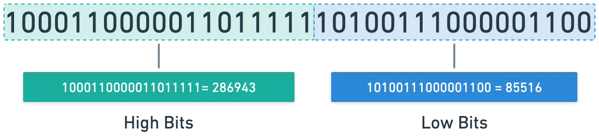
Compression works by taking some number $2^d$ and performing two operations:

• Divide each coefficient of $W(X)$ by $2^d$, and round down. The result is called the high bits.
• Then, calculate $\textrm{mod} \ 2^d$ for each coefficient of $W(X)$. These are called the low bits.

The naming might seem strange at first. But everything makes sense when you realize that the binary representation of $2^d$ is just a $1$ followed by $d$ zeros!

And this works very nicely when calculating the two operations above dividing is the same as shifting the bits $d$ spaces to the right, and mod can be calculated by taking the $d$ last digits of a number.

Don’t believe me? Let’s work out an example together:

• Take the number $37610278412$. Its binary representation is $100011000001101111110100111000001100$ (see here).
• Next, choose a power that gives roughly half the digits of the number we selected before. In this case, let’s use $17$. So, $2^{17} = 131072$.
• We calculate the high bits as $⌊37610278412 / 131072⌋$, which yields $286943$. The binary representation is $1000110000011011111$.
• Finally, we calculate the high bits as $37610278412 \ \textrm{mod} \ 131072$, which gives a result of $85516$; in binary, $10100111000001100$.

And now, just like clockwork:

Click to zoom

Okay, that was quite a lot! Let’s just pause a moment and appreciate how beautifully simple this process is!

In Dilithium, we only keep the high bits of every coefficient in the vector of polynomials $w$ — we’ll denote this result $w_1$.

If you’re like me, you’re probably feeling like this at this point in the article:

The good news is we’re very close to the finish line! Take a couple of deep breaths. This will only take a few more minutes.

Whenever you’re ready, let’s move on.

Signing, Part Two

We have the compressed nonce commitment — but that’s just the first part of the signature. Imagine the signer sends this commitment to the verifier, and in response, the verifier sends some challenge $c$, which is just a small polynomial with coefficients $-1$, $0$, and $1$.

With it, we calculate the final signature value, which is:

$$z = y + c.s_1 \ \textrm{mod} \ q$$

And the signature is just the tuple $(z, w_1, c)$.

There’s an important extra bound verification step here, but we’ll skip that in the interest of simplifying things a little.

Now, you may have noticed two things: one, the signature doesn’t include the message anywhere, and two, as I described it, this would be an interactive protocol, which is something we don’t want.

We already know that using the Fiat-Shamir transform, this can be turned into a non-interactive signature scheme by means of a hash. And by throwing the message into the mix, all our requirements are satisfied!

So we just need to calculate the hash (Dilithium uses a hashing algorithm called SHAKE, part of the SHA-3 family) of the compressed nonce and the original message:

$$c = H(w_1, M)$$

This is just a binary number, though — we need to convert it to a polynomial with coefficients $-1$, $0$, and $1$. To achieve this, the technique we use is called rejection sampling. Which, simplifying a bit, could look like this:

• $00$ maps to $0$
• $10$ maps to $1$
• $01$ maps to $-1$
• $11$ is not considered valid, so we discard the value and move on to the next two bits.

In reality, this mapping is a bit more complex to ensure that most coefficients are $0$.

The hash kinda works as a sampling of a random distribution from which we take samples, reading the stream of data 2 digits at a time, generating one coefficient of c at each step.

Cool! Our signature is done and dusted. How does verification work?

Verification

Quick recap: the verifier holds a public key $(A, t)$ and now also holds the signature $(z, w_1, c)$ to the message $M$.

To verify, they just need to compute:

$$w' = A.z - c.t \in R^k$$

Substituting the correct value of $z$ here yields:

$$w' = A.y - c.s_2 \in R^k$$

Essentially, $w’$ will be different from the original commitment $w$, but the difference is just a vector of small polynomials $c.s_2$ — just some small noise.

Another way to say this is that only the low bits of polynomial coefficients will be different from one another when comparing $w$ and $w’$, while the high bits should match. Would you look at that! Nothing short of sorcery.

The verifier just needs to calculate the high bits of $w’$ and compare that result with with $w_1$. Should they match, the signature is accepted!

Again, the bound check is also important to prevent forgery, fully harnessing the hardness of the Shortest Vector Problem (SVP) in a lattice, but we’ll skip that part here.

The original paper goes into full detail about this. And for an alternative look at Dilithium, here’s another article with a slightly different perspective.

Summary

What a ride, eh?

These are only two of the new methods in the surging world of post-quantum cryptography. Not all methods being proposed are based on lattices, though. There’s a lot of information to take in out there, and probably lots of amazing research to read (that I still need to go through!).

Still, lattice-based cryptography looks promising as the next generation of standard cryptographic algorithms.

Moreover, part of the appeal of using lattices is related to their features, something we haven’t talked about yet. Because everything is based on rings behind the scenes, and since rings support two operations, this is fertile soil for something super cool: fully homomorphic encryption, or FHE for short. This will be the topic for the next (and probably the last) article in this series.

Until next time!