Cryptography 101: Ring Learning With Errors

This is part of a larger series of articles about cryptography. If this is the first article you come across, I strongly recommend starting from the beginning of the series.

In our previous installment, we introduced yet another structure for us to play with: rings. These will open the path for some cryptography that’s fundamentally different than anything we’ve seen so far.

Let’s not get ahead of ourselves, though — there’s one more thing we need to do before trying to understand any new cryptographic technique.

No method is usable in practice unless it’s secure, so to speak. At this point in the series, we know full well that security is measured in terms of how hard it is to break a scheme.

To answer this, we need to understand the associated mathematical problem that is assumed to be hard. We’ve seen a couple so far in the series — like the integer factorization problem and the discrete logarithm problem.

Of course, there are more such problems. Today, we’ll be learning about a brand new one, which will be the backbone for ring-based cryptography.

Alright, let’s see what we’re working with!

Setting Things Up

Ring Learning With Errors (RLWE for short) is a problem based on polynomials. A quotient polynomial ring, to be precise. As a short refresher, this means that we’ll be working with some ring:

$$\mathbb{F}_q[X]/(f(X))$$

Such that we can reduce any polynomial modulo $f(X)$ — the modulus polynomial.

We explained this in detail in the previous article, so go check that out if need be!

Now... What can we do with this?

Let’s try to develop our understanding step by step. Given a couple polynomials $A(X)$ and $S(X)$, we can calculate their product, like so:

$$B(X) = S(X).A(X)$$

The ring properties come into play at this point: $B(X)$ is reduced modulo some polynomial $f(X)$ of choice, ensuring that the degree is always bounded.

Here’s a question for you: if I give you $B(X)$ and $A(X)$, how hard do you think it would be to recover $S(X)$?

Well, it’s not that hard at all!

Turns out, with a careful choice of $f(X)$, every polynomial in the ring can be inverted. It works exactly like modular inverses in finite fields: for every polynomial $P(X)$, we can find some $P^{-1}(X)$ such that:

$$P(X).P^{-1}(X) \ \textrm{mod} \ f(X) = 1$$

Having this tool makes the task really simple: you just find $A^{-1}(X)$ and compute:

$$S(X) = B(X).A^{-1}(X)$$

Okay, this doesn’t seem like a good candidate for a hard problem. Or does it? How about we modify it a little?

Switching It Up

With just a nudge in the right direction, we can transform this seemingly innocent and easy-to-solve expression into something much more useful. It’s really quite simple — all we need to do is throw some error or noise polynomial into the mix:

$$B(X) = S(X).A(X) + E(X)$$

The error needs to be small — just a little noise is enough, as we’ll see further below.

That’s all! Quite the unusual plot twist, given the crazy stuff we’re used to.

This rather inconspicuous adjustment hides a lot of complexity. Let’s ponder this expression for a moment.

Reorganizing the expression a little yields:

$$E(X) = B(X) - A(X).S(X)$$

Looking at it from this perspective, it’s easy to see that given any polynomials $A(X)$ and $B(X)$, we can basically choose any $S(X)$ and calculate $E(X)$. What this means is that there’s no unique or direct way to relate $A(X)$ and $B(X)$. The solution is no longer straightforward.

Sounds promising!

But before we move on to an example, there’s something we need to talk about. What’s the learning in “learning with errors”?

The Learning Problem

For this section, we’re gonna need to change perspectives again. Don’t worry — nothing strange. Things will be pretty friendly this time around.

Instead of the polynomials $A(X)$ and $B(X)$ themselves, let’s work with their evaluations. So, we’ll choose some values for $X$ and calculate:

$$a = (A(x_0), A(x_1), A(x_2), ..., A(x_{n-1})) \in {\mathbb{F}_q}^n$$ $$b = (B(x_0), B(x_1), B(x_2), ..., B(x_{n-1})) \in {\mathbb{F}_q}^n$$

These vectors are clearly related — they follow the polynomial equation we described before:

$$b = a \cdot s + e \ \textrm{mod} \ q$$

Where $a \cot s$ is component-wise multiplication.

As always, the question is, why would this be helpful? The answer will become clearer as we explore some applications! Bear with me for a moment.

The problem is now stated as follows:

Given $a$ and $b$, find $s$.

In the same vein as the previous discussion, this is really hard as long as e is carefully chosen — meaning that it’s randomly sampled from a specific distribution. Picture something akin to a normal distribution.

What makes this hard is that, because of the addition of the noise vector $e$, it’s really complicated to tell whether if $b$ is just a random vector or if it was indeed calculated as $b = a \cdot s + e \ \textrm{mod} \ q$. Conversely, it’s really hard to determine $s$ with knowledge of $a$ and $b$. As long as $s$ and $e$ are not revealed, of course.

These two versions of the same coin are known as the decision problem and the search problem. Most problems in cryptography can be written as either version — they are equivalent.

Ok, cool. Now what? Having a hard problem is not fun unless we can build something with these new gadgets!

Building An Example

We’ll be building something based on this paper, which is one of the foundational works in this area.

Let’s imagine we want to encrypt a message. Typically, we’d approach this by generating keys and use them to apply some operation on the message that can later be undone by the receiver. And that’s exactly what we’ll do.

Encryption

Our key will just be a randomly-sampled polynomial $s(X)$. For simplicity, let’s just write $s$. Then, we need a message to encrypt. For our intents and purposes, this will be another polynomial, which will be denoted by $m$. Its coefficients are bounded between $0$ and some integer $t$, lower than $q$.

For instance, $t$ can be $2$ so that the coefficients are actually a binary sequence.

Encryption is really simple: we just sample a couple of polynomials $a$ and $e$, and calculate:

$$c_0 = a.s + t.e + m \ \textrm{mod} \ q$$ $$c_1 = -a$$

The pair $(c_0, c_1)$ constitutes the ciphertext. These can be sent to a receiver, which will now attempt to recover the message with knowledge of s. Because of this, it’s a symmetric encryption algorithm.

Decryption

Upon receiving the message, the receiver will simply calculate:

$$m = c_0 + c_1.s \ \textrm{mod} \ t$$

Yup! It’s that simple.

Here, let’s do the math and verify that this works. Substituting $c_0$ and $c_1$ leaves us with:

$$(c_0 + c_1.s) \ \textrm{mod} \ t = (t.e + m) \ \textrm{mod} \ t = m$$

As you can see, the error magically disappears because the operations are performed modulo $t$. Wonderful!

If we compare these two expressions:

$$m = c_0 + s.c_1$$ $$B(X) = E(X) + S(X).A(X)$$

You can probably spot the parallel between this and our first formulation of the problem. Anyone seeing the ciphertext without knowledge of $s$ would not be able to tell $c_0$ and $c_1$ apart from random polynomials.

Essentially, they’d have to solve the RLWE problem. And we already know — that’s freaking hard to do!

Here’s a link to an even simpler example of encryption, where we encode a single bit. The example is based on some things we’ll discuss further ahead — but if you yearn for something more interactive or need a break from reading, maybe go check that out!

There will be time for us to explore more methods later. For now, it’s important to put that on hold and instead explore a very interesting connection.

Lattices

Woah woah woah. What?

We were just talking about polynomials, and you now bring up lattices? What’s even a lattice?

Okay, you’re right, we need some context. Although we haven’t yet defined what a lattice is — nor their connection with rings — what I can say is that many PQC methods are based on problems on lattices. And so it’s important to understand what they are. Studying their connection with RLWE might also provide us with some insight to evaluate their security.

With that, we’re ready for some definitions.

What is a Lattice?

Take a point in two-dimensional space. Now, draw two vectors like this:

Click to zoom

Of course, to be usable in cryptography, these vectors need to have integer values.

With this, we start an iterative process.

Place a point at the end of each vector. Using them as starting points, repeat the process. Oh, and also do the same thing in the opposite direction of the original vectors.

What you end up with is an infinite set of points that are evenly spaced, as if creating an infinite pattern. This is a lattice generated by our two basis vectors.

Click to zoom

By the way, when working with finite fields, these lattices are not infinite — they are reduced modulo $q$, as you’d expect.

Alright, alright. Another toy to play with! But we know that this is no good for cryptography unless we can propose a hard problem around it.

The Lattice Problem

With the vectors in the image above, it’s pretty easy to spot a pattern in the lattice. Imagine I give you some random point that’s not on the lattice — because the pattern is simple, it’s pretty easy to tell which lattice point is the closest to the one I gave you:

Click to zoom

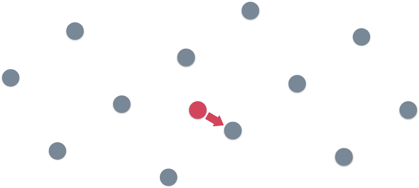
A question for you: is it always so easy?

Pause for thinking.

.

.

.

.

.

.

. ☕️ A coffee always helps.

.

.

.

.

.

.

Okay, that’s more than enough!

The answer is that it depends. It depends on the basis vectors we choose, and in some cases, the emerging pattern will not be as simple. Like in the following example:

Click to zoom

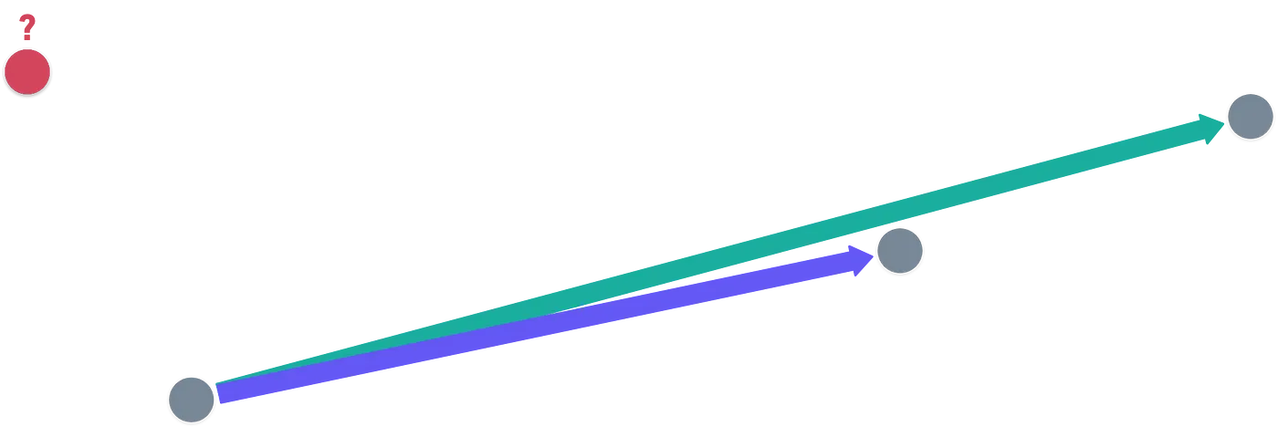
The infinite pattern is not as simple to spot now. And the way to find which is the closest lattice point to the red point is to start trying combinations of the basis vectors until we get a good candidate. But… How can we be sure that our candidate is the closest point in the lattice?

This problem called the Shortest Vector Problem, or SVP for short. And it’s damn hard. Generally speaking, difficulty increases because of two things:

• How collinear the basis vectors are — or how close to parallel they are.
• The number of dimensions in which we define the lattice.

Oh, yeah, because we’re not bounded to two dimensions. Did I forget to mention that? It’s not uncommon to use lattices in hundreds or even thousands of dimensions.

Click to zoom

We can use as many as we need to! And that makes the problem really, really hard.

Wait, stop. Hold on a second. Weren’t we looking for a connection with RLWE? We don’t want to stray too far from our main goal. How is this all connected, then?

RLWE and Lattices

We started working with polynomials, and now we’re dealing with vectors. These constructions seem to operate on entirely different worlds — but in reality, they aren’t so far apart. Take a look at this:

$$P(X) = p_0 + p_1X + p_2X^2 + ... + p_{n-1}X^{n-1}$$ $$p = (p_0,p_1, p_2, ..., p_{n-1})$$

See what we did there? We just wrote the coefficients of the polynomial as a vector! You’ll find that adding these vectors is equivalent to adding the associated polynomials.

With this new insight, let’s examine our original hard problem in RLWE, again:

$$E(X) = B(X) - A(X).S(X)$$

Imagine $B(X)$ is a vector, representing a point in n-dimensional space. We need to find $S(X)$ such that $A(X).S(X)$ is the closest it can be to $B(X)$. In consequence, $E(X)$ will be the smallest possible difference between these polynomials — and applying our previous equivalence, it’s the shortest possible vector.

Ahá! This is shaping up nicely! By thinking of the noise polynomial as a short vector, at least the final goal of both problems seems interchangeable!

Nevertheless, there appears to be an issue: how is the expression $A(X).S(X)$ related to searching for points on a lattice? If we can tie this loose end, then we’ll get the full connection between these problems.

This one is not as straightforward. It’s the final stretch — please bear with me just a little longer!

Remember ring ideals? Those pesky thingies that were super abstract to define? We’ll need them here!

The polynomial $A(X)$ is used to define an ideal in our polynomial ring of choice. It’s defined as:

$$I = \{A(X).S(X) \ \textrm{mod} \ f(X) \ / \ S(X) \in \mathbb{F}_q[X]/(f(X)) \}$$

This is a two-sided ideal, since commutativity holds in polynomial rings.

We already know how an ideal can be used to calculate a quotient ring. All that remains is to map each polynomial in the ideal to a vector — and right there my friends, we’ve just found ourselves our lattice!

These are often called ideal lattices, because of how they originate from an ideal of the polynomial ring.

Interestingly, the basis vectors for this lattice can be calculated by taking $A(X)$ and multiplying it by $X$ successively. And in some special cases (like when using cyclotomic polynomials), the basis ends up being a rotation of the coefficients of $A(X)$.

For example, using the polynomial $A(X) = a_0 + a_1X + a_2X^2$, and working with the ring $\mathbb{F}[X]/(X^3 + 1)$, then the basis for the ideal lattice is formed by the vectors $(a_0, a_1, a_2)$, $(a_2, a_0, a_1)$, and $(a_1, a_2, a_0)$.

Summary

I think that’s more than enough to have an initial grasp of the structures that underpin most post-quantum methods.

There’s much more to RLWE and lattices out there, of course! But we’ll have to be content with this much, at least for now.

Most of the time, the goal for this series is not to go into full rigorous detail about every structure or construction we present — what I consider most important here are the general concepts and ideas we discuss.

Our main takeaway from this article should be the RLWE and SVP problems, and also the rough concepts of how rings and lattices work in practice.

That will be all we need to explore some PQC methods — we’re now ready to get to the good stuff!

Presenting some of these methods will be the topic for next article. See you soon!