Cryptography 101: Fully Homomorphic Encryption

This is part of a larger series of articles about cryptography. If this is the first article you come across, I strongly recommend starting from the beginning of the series.

We’re here. The very end of the journey.

We’ve learned a lot along the way. What started as a rather simple intro to groups ended up turning into a full-blown series, where we explored many fundamental ideas in cryptography, but also some techniques that are very close to being state-of-the-art. I’m quite happy with the result.

However, there’s one important subject we haven’t touched upon so far. It’s nothing short of a holy grail in cryptography. And by now, we have all the right tools to understand how modern techniques approach this problem.

That’s right. It’s time to dive into Fully Homomorphic Encryption.

Introduction

Homomorphic is a term we should already be familiar with, as we dedicated an entire article to explaining its meaning. Still, a short refresher never hurts.

An homomorphism is a type of function, which has this simple property:

$$f(a + b) = f(a) +_f f(b)$$

Note the subtle distinction that the operations need not be the same.

In plain english: the result of adding the inputs first and then applying the function is the same as if we invert the order.

Really, we say that the function is homomorphic with respect to some operation, which in the above scenario, happens to be addition.

Some homomorphisms are also invertible, meaning that for some functional value $y = f(x)$, there’s some inverse function such that:

$$f^{-1}(y) = x$$

In this case, the function is called an isomorphism instead.

Some encryption functions behave like isomorphisms. Being able to reverse encryption is a requirement for the functionality, but the fact that it behaves like an homomorphism unlocks some new superpowers.

Namely, you can add encrypted values, and have the guarantee that when decryption happens, you’ll get the same result as if you added the unencrypted values first. And that’s very cool — it allows applications to perform operations on encrypted data, thus preserving privacy.

Click to zoom

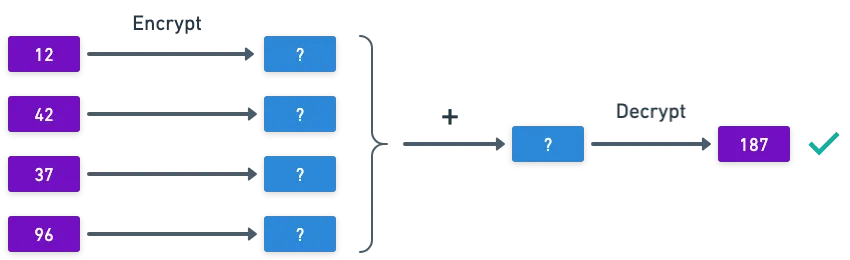
There’s a catch, though: when working with groups, we can only support one operation.

As a consequence, we can create group-based encryption methods that can handle addition of encrypted values quite easily (i.e. ElGamal). But you want multiplication? Nope. Can’t do that.

Supporting multiplication is important — as we saw in our brief pass through arithmetic circuits, we can calculate just about anything with addition and multiplication gates. This means that if we could support both operations, then we could perform arbitrary computations over encrypted data, while keeping the data private!

The family of algorithms that support a single operation was baptized as Partially Homomorphic Encryption, or PHE.

Importantly, this might be enough for some types of applications. For example, in case we only need to keep encrypted balances and add or subtract from them, we don’t require the full power of FHE.

Turns out that a method that supports both addition and multiplication was not easy to conceive. For a long time, it remained elusive for researchers. There were efforts like the Boneh-Goh-Nissim algorithm, based on pairings, which could handle a single multiplication.

It was simply not enough. Supporting two operations remained out of reach.

But wait... Two operations? We know a better structure for that!

Encryption With Rings

Rings sound like the algebraic structure that should naturally support fully homomorphic encryption. Efforts such as NTRU were initially proposed, but could only handle a limited amount of multiplications. And there’s good reason for this.

In the previous article, we looked at Kyber, which can be used to encrypt short messages. When looking at the decapsulation (think decryption) step, we observed that the recovered message was not exactly the original message.

But it was close to it. Off by only a small error. Decryption will be possible as long as this error is kept small.

This is the idea behind what’s colloquially called Somewhat Homomorphic Encryption, or SWHE: methods that can handle decryption as long as the error remains small.

And although Kyber is not an homomorphic encryption method, the idea is roughly the same.

Multiplications have a tendency to blow errors up, and that’s the reason why ring-based methods could not support an unlimited amount of them. At least that was the case, until something remarkable happened...

In 2009, Craig Gentry published his PhD thesis, which introduced a couple new techniques that unlocked the first ever truly FHE scheme.

As his original work suggests, research started with an initial construction, on top of which some techniques were applied that transformed his base SHE scheme into a FHE one. I think the best approach here is to follow the same steps!

Base Construction

Everything starts with an adequate ring choice. We’ll be working with rings of the form $\mathbb{F}[X]/(f(X))$. And we also need an ideal for said ring — remember that an ideal is a subset of $R$ which is closed under addition and multiplication by any element of $R$:

$$x, y \in I \Rightarrow x + y \in I$$ $$x \in I, r \in R \Rightarrow r.x \in I$$

The ideal is generated randomly. A random polynomial $g(X)$ with small coefficients is sampled — and then, the ideal is just $(g(X))$, much like we explained here.

To continue, we must again talk about the notion of a basis. We touched upon this concept a couple articles ago. Simply put, a basis consists of a set of independent vectors which can be used to produce any point in the lattice via linear combination. We say a basis generates a lattice $\Lambda$.

$$\Lambda = \left \{ \sum_{i=1}^n z_i.b_i \ | \ z_i \in \mathbb{Z} \right \}$$

Bases for a lattice are not unique, and there are several valid bases we could choose. As we already hinted in previous articles, there are good bases and bad bases — the good ones allow for quick solving of the Shortest Vector Problem (SVP), while the bad bases, even though they generate the same lattice, are not good for efficiently solving it.

Click to zoom

From the image, we can imagine that a good basis should be a set of short, non-collinear (orthogonal, if possible) vectors. On the other hand, bad bases will be just the opposite: long, collinear vectors.

And so, in the construction that we’ll be looking at, two bases are generated — they serve as the private and public keys for the encryption process:

$${B_J}^{sk}, {B_J}^{pk}$$

The secret key is a "good" basis, while the public key is a "bad" one.

It should be noted that we're referencing an ideal $J$ here, not $I$. This is not a typo - there's good reason for this. Let's just work through the problem setting slowly. Really, all that happens is that the bad basis is only good for calculating an encrypted value, but really inefficient to decrypt - while the good basis allows for fast computation during decryption. That's enough detail for us here - there are other more pressing concepts for us to understand!

Encryption

As per usual, encryption starts with a message. One point we often avoid defining clearly is what set valid messages belong to - or in other words, what the plaintext space is. In our case, valid plaintext values will belong to the quotient ring $R/I$. Two things are noteworthy here:

• We need a way to encode messages into ring elements — but we can skip that part for now.
• We also need to understand what an element of $R/I$ is. More on that in just a minute.

Next, and again as usual, we need to introduce some randomness into our encryption scheme. This ensures that when encrypting the same value $m$ twice, we get two different results.

A random nonce is chosen from the ideal $I$, with the aid of a basis $B_i$. The resulting ciphertext $\psi$ will be the original encoded message $m$, plus the sampled nonce $i$:

$$\psi = (m + i) \ \textrm{mod} \ {B_J}^{pk}$$

Using ring-specific lingo, notice that $m + i$ is essentially a random element of the coset $m + I$ — this is, all the elements of $R$ that have the form:

$$m + I = \{ m + i \ | \ i \in I\}$$

If this seems confusing, it’s because it is. And since this is the last stretch in the series, I’ll try to explain this in more detail via a couple examples.

Visual Aid to the Rescue

Suppose we’re working with the ring $\mathbb{Z}[X]/(X^2+1)$. Every polynomial in the ring will have degree at most 1—meaning that we can represent polynomial coefficients in a plane, as 2D vectors.

The first coordinate corresponds to the constant term, and the second one to the first degree coefficient (the number multiplying $x$).

We then choose a basis $B_i$ for an ideal $I$ — this is, two vectors that determine an ideal. Let’s choose for example the polynomials $x + 2$ and $2x - 1$; we can associate them with the vectors $(2,1)$ and $(-1,2)$ in two-dimensional space:

Click to zoom

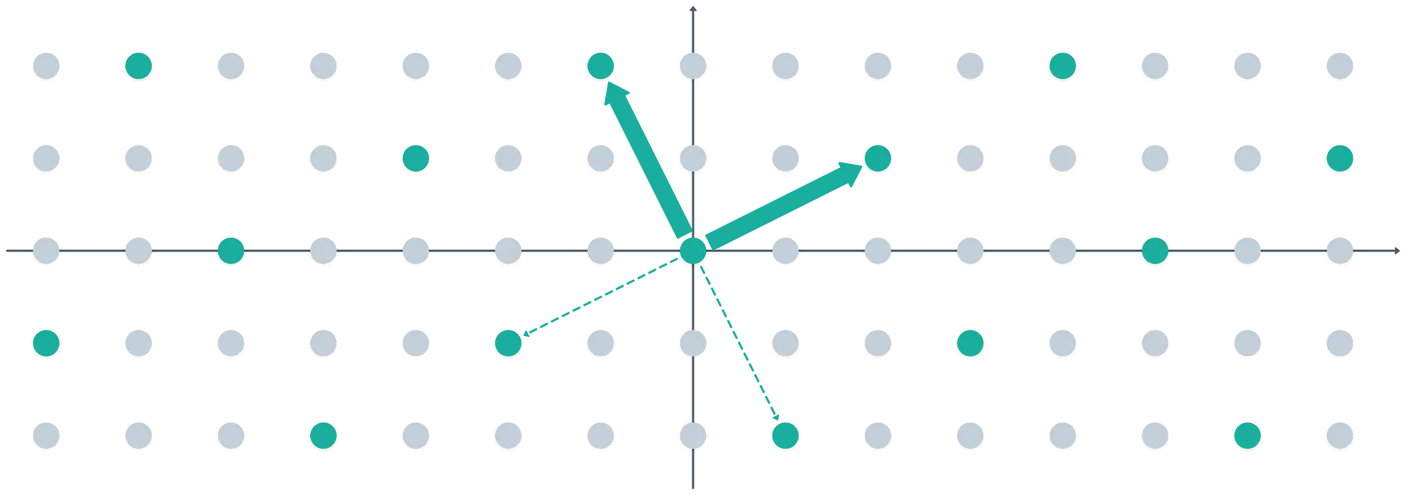
The choice of basis hides an interesting subtle detail. The second element was calculated as $x(x+ 2) = x^2 + 2x$. But in the ring we’re using, $x^2$ is equivalent to $-1$!

Multiplying by $x$ has the nice property of rotating vectors in the ring. That’s why we got a nice pair of orthogonal vectors.

Every point in the image (both the light and dark grey ones) is an element in the ring $\mathbb{Z}[X]/(X^2+1)$. And it’s easy to see the ideal in action here: not every point in the ring is included in the ideal lattice.

To better understand cosets, just take a different initial point, and use the same basis vectors to generate a lattice:

Click to zoom

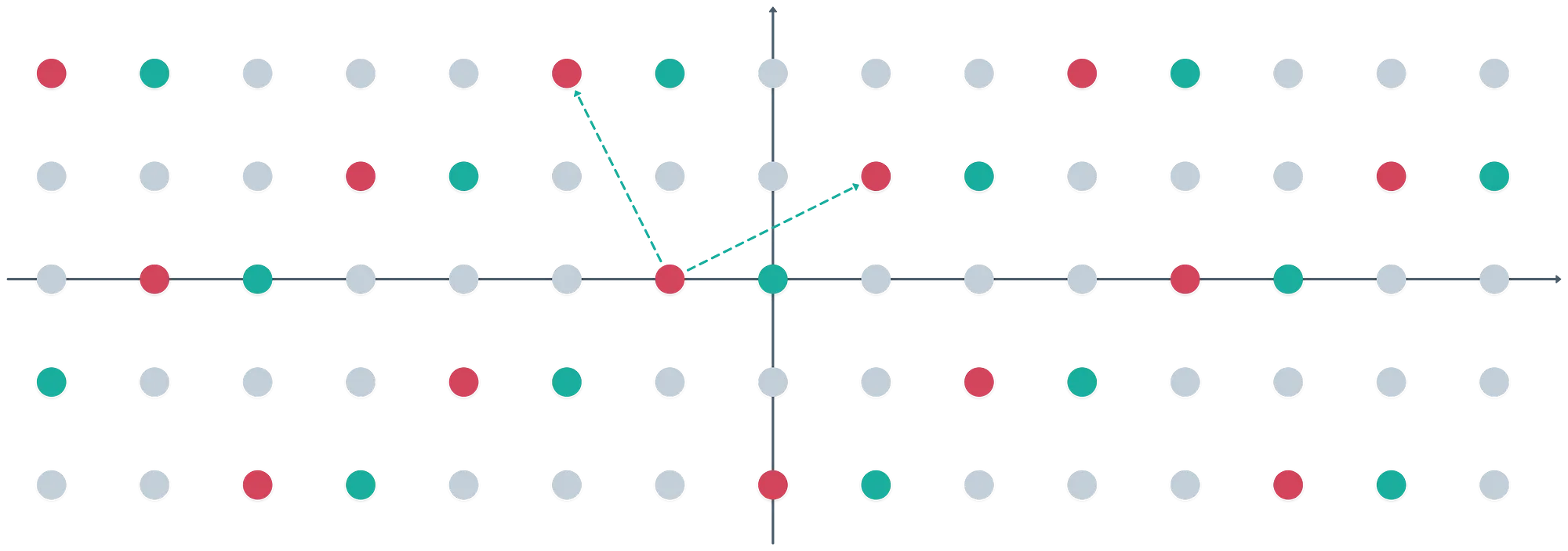
Do you see what just happened? We get essentially the same pattern, but shifted. These are the cosets we’re talking about. Interestingly, each coset can be identified by just a single element in it — then, all the other elements are generated by adding linear combinations of the basis vectors.

In fact, the quotient ring $R/I$ is made up of these distinct cosets. It’s just that a single representative is enough to identify the entire coset, which is also an equivalence class.

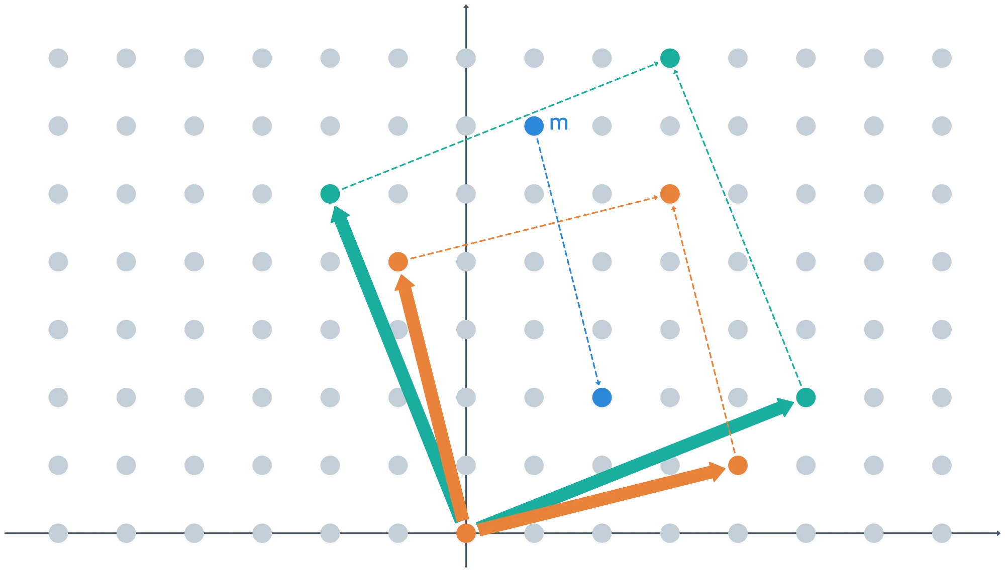
Finally… What does it mean to take $\textrm{mod} \ B_i$? It’s pretty simple, actually: any vector in our ring $R$ can be represented as the sum of linear combinations of the basis vectors, plus an extra short vector that allows us to move “away” from the ideal:

Click to zoom

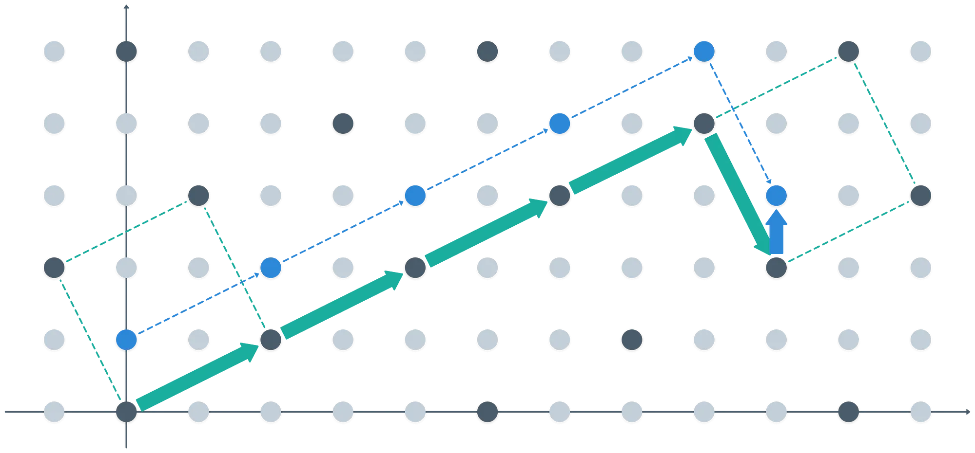
We can think of the blue vector as a remainder, thus being the result of taking $\textrm{mod} \ B_i$ on any point in the ring. But it’s also a representative for a coset!

Formally, what happens is that taking $\textrm{mod} \ B_i$ on any point in the ring $R$, maps it to the respective equivalence class in $R/I$. Thus, these two are equivalent:

$$R / I = R \ \textrm{mod} \ B_I$$

And the representatives for the cosets are usually elements of the fundamental parallelepiped determined by the basis, which is highlighted by the green dashed lines in the image above.

This should not be all that unfamiliar — it’s essentially the same situation we described for the ring of integers modulo $q$:

$$\mathbb{Z}/(q) = \mathbb{Z}_q = \mathbb{Z} \ \textrm{mod} \ q$$

And to cement this idea, look at what happens when we paint all the cosets in the previous example:

Click to zoom

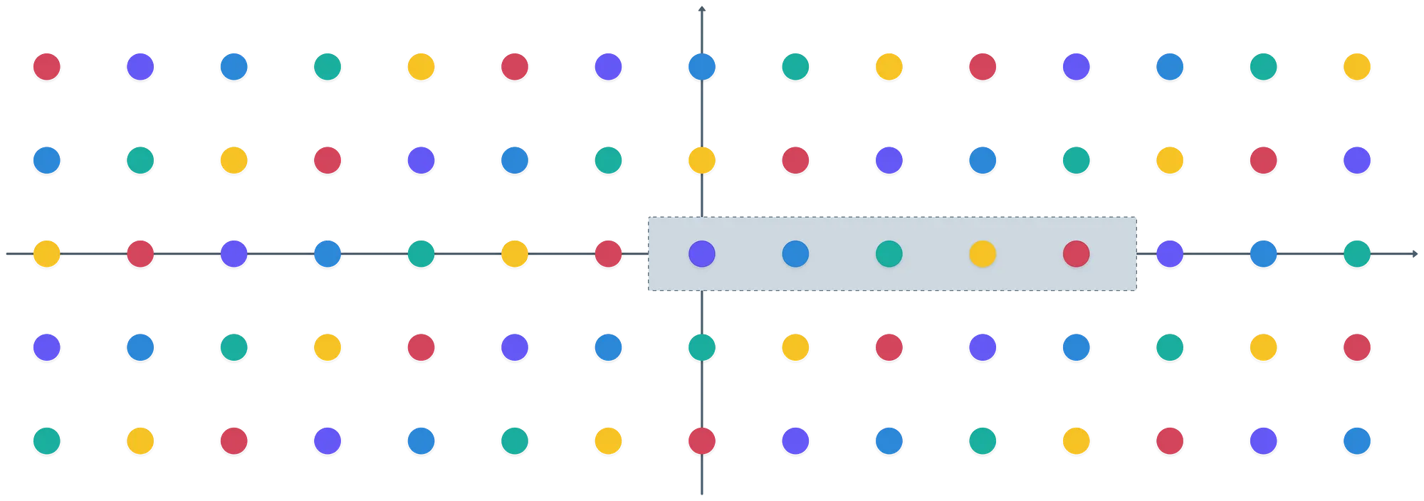
Each element in $\mathbb{Z} \ \textrm{mod} \ q$ happens to map to a different coset in $R/I$, as we can see in the grey box — and $q = 5$, which is the number of distinct cosets.

Cool! How are we feeling so far?

Good news is that after these concepts are understood, we can at least interpret the encryption and decryption processes!

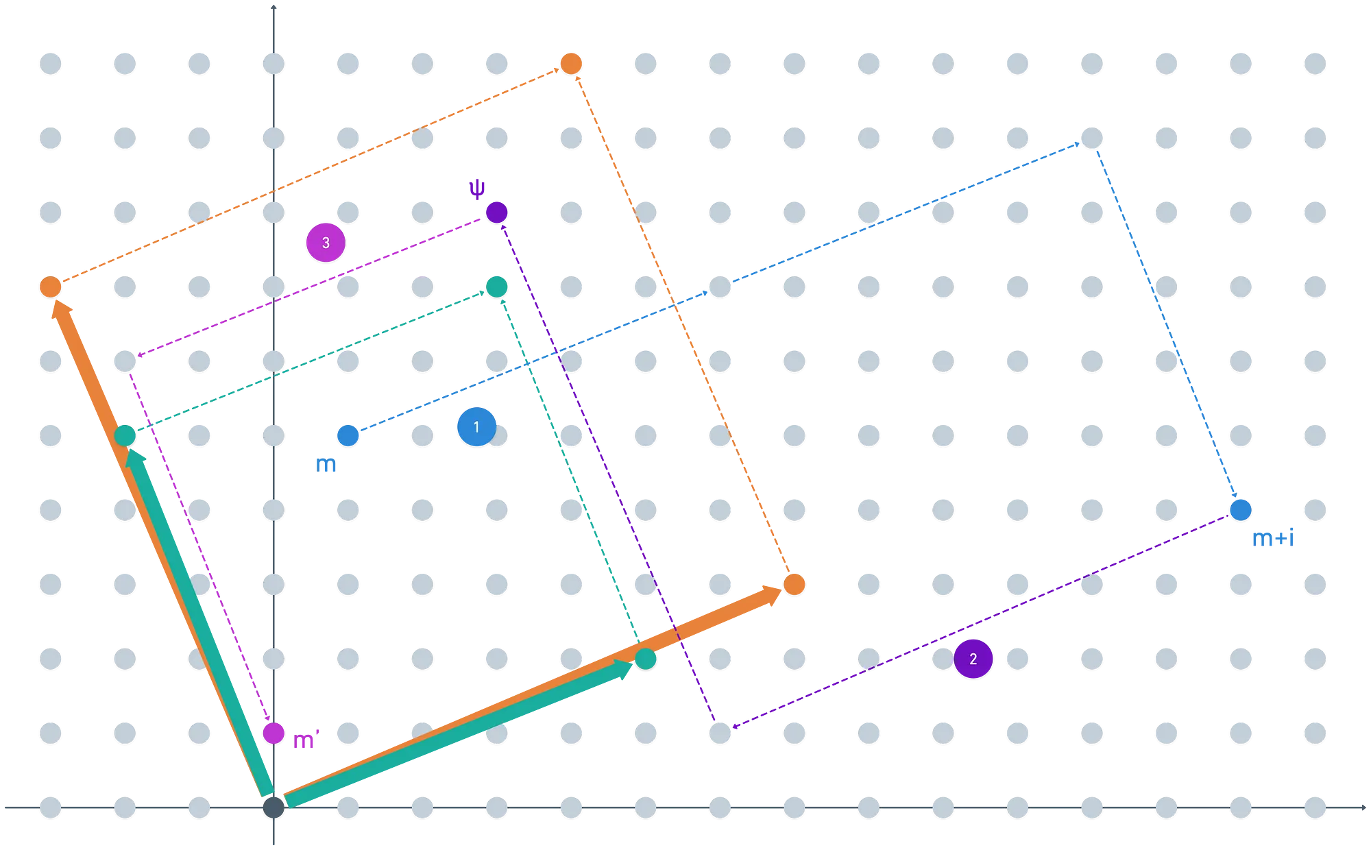
Let’s focus on the encryption function again:

$$\psi = (m + i) \ \textrm{mod} \ {B_J}^{pk}$$

We’re in condition to interpret a few things now:

• $m$ represents a coset in $R/I$.
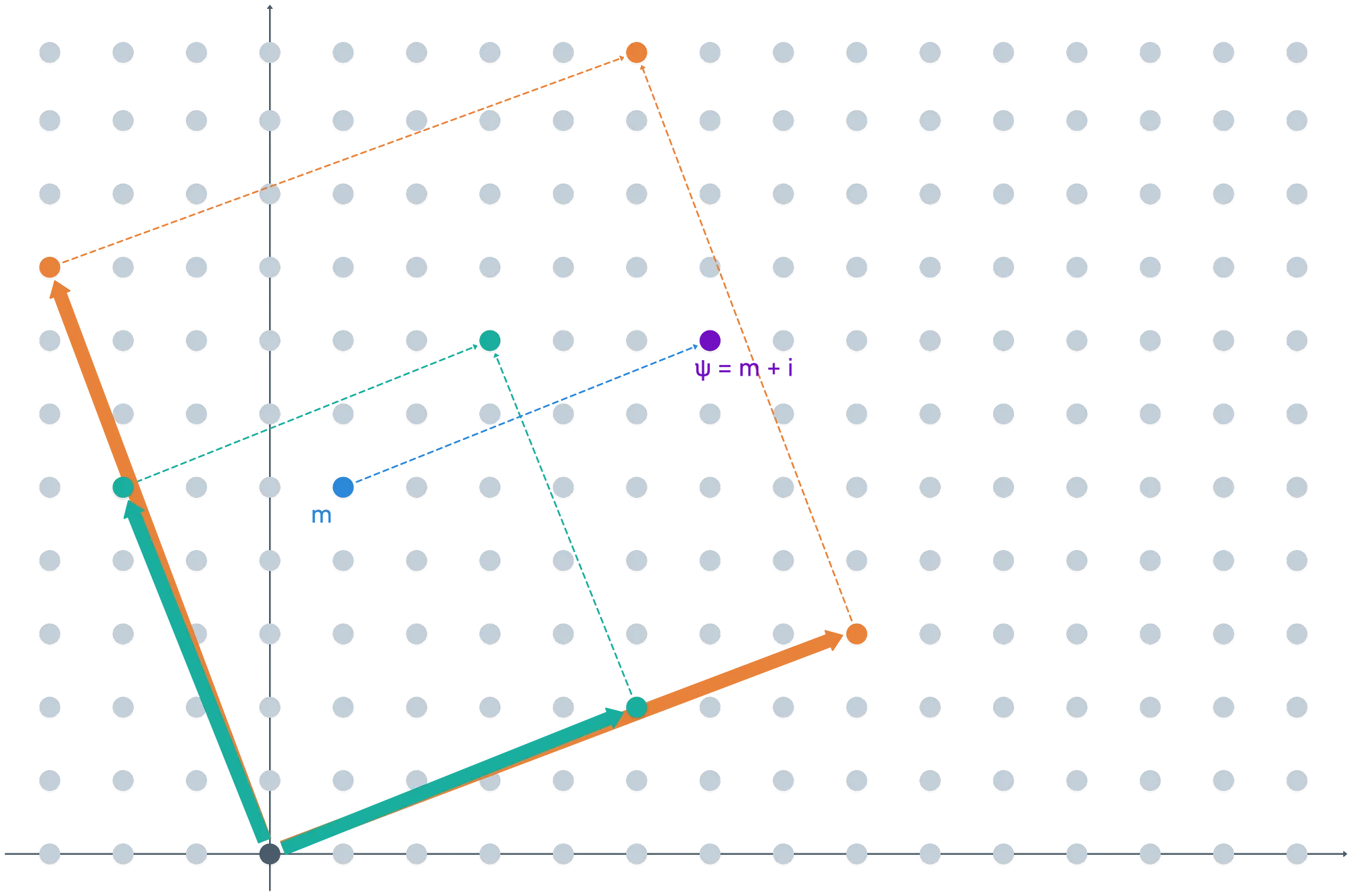
• $m + i$ is just another representative for the same coset. We can clearly see how the plaintext space is meant to be $R/I$.
• However, taking $\textrm{mod} \ B_j$ changes things a bit: the result will be a coset representative of $R/J$.

We haven’t talked about $J$ yet, have we?

The ideal $J$ is different from $I$, in such a way that using any basis for $J$ in combination with a basis for I allows us to get any element in the ring $R$. This is sometimes expressed as $I + J = R$, and we say that $I$ and $J$ are coprime.

Because of this, $i$ (which is just a linear combination of the basis elements of $I$) essentially adds some noise to $m$. What I mean is that these two expressions generally don’t yield the same result:

$$m \ \textrm{mod} \ {B_J}^{pk} \neq (m + i) \ \textrm{mod} \ {B_J}^{pk}$$

We’ll see this in action further ahead.

Decryption

Decrypting the ciphertext $\psi$ is as simple as taking a couple modulo operations:

$$m = (\psi \ \textrm{mod} \ {B_J}^{sk}) \ \textrm{mod} \ B_I$$

What’s not that simple is understanding why. Let’s focus on the simplest scenario for a moment:

$$\psi = m \ \textrm{mod} \ {B_J}^{pk}$$

So, no added noise.

Also, let’s assume for a moment that both bases for $J$ are equal, and let’s see what happens with an example, again.

$$I = (5 + 2x) \Rightarrow B_I = \{(5,2), (-2,5)\}$$ $$J = (7 + 3x) \Rightarrow B_J = \{(7,3), (-3,7)\}$$

Take a message $m$ inside the fundamental parallelepiped of $I$ (the shape defined by the basis vectors):

Click to zoom

Because m is inside the fundamental parallelepiped of both $I$ and $J$, then taking modulo during encryption and decryption will for sure yield back $m$. What happens if $J$ is “finer”, though?

Click to zoom

Notice that taking the first modulo operation maps the message into a new coset of $R/I$ — which is something we don’t want! If this happens, we’d get back a different message upon decryption. In this sense, we require $J$ to be sort of coarser than $I$.

Now, let’s add some noise $i$ to the original message, and use our original $J$. What happens in this case if we follow a full encryption / decryption cycle?

Click to zoom

As you can see… We don’t get back the original plaintext.

What’s wrong here?

Actually, what we just witnessed is at the core of the whole fully homomorphic deal: our error was too big. If we keep it a little smaller, things will work out just fine:

Click to zoom

During encryption, we’ll most likely get an element in the coset of $J$ represented by $\psi$. We don’t really care that it’s inside the fundamental parallelepiped, just that the value represents the same coset. And that’s also closely tied to why we use two bases!

Cool, that settles it: as long as the noise is small, we can decrypt, no problem. But remember, this article is not about encryption alone — it’s about fully homomorphic encryption. What happens when we start performing some operations?

Homomorphic Operations

For the scheme to be fully homomorphic, we must be able to support both addition and multiplication. They behave roughly like this:

$$\psi_1 + \psi_2 = (m_1 + m_2 + i_1 + i_2) \ \textrm{mod} \ {B_J}^{pk}$$ $$\psi_1.\psi_2 = (m_1.m_2 + m_1.i_2 + m_2.i_1 + i_1.i_2) \ \textrm{mod} \ {B_J}^{pk}$$

The total noise during addition seems to grow in a manageable way, but multiplication blows noise out of the water really fast. And this complicates things: it means that after a few multiplications, errors may grow to a point where decryption is no longer possible. As it stands, this is a Somewhat Homomorphic Encryption scheme — it can handle a maximum amount of operations.

It’s still “better” than most other efforts prior to this technique, in the sense that it can theoretically handle more than one multiplication!

As if things were not complicated enough… Oh boy.

Hold tight!

Managing Errors

When performing operations, errors are going to grow no matter what. It’s a parameter that seems to be out of our control — an intrinsic property of the scheme, if you will.

But there is something we can do to keep them in check. This is the idea behind Gentry’s thesis: a scheme that allows refreshing the errors that are almost too big, and obtain an error that is “shorter”.

Obviously, the error could be reduced if we were allowed to decrypt the message — you just need to choose a new, small noise vector. But of course, the whole gist of the matter is doing this without decrypting. That’s where things get interesting. In Gentry’s own words:

“we do decrypt the ciphertext, but homomorphically!”

I know, sounds crazy! To give a rough idea of what this means, let’s call the encryption function $\mathcal{E}$ and the decryption function $\mathcal{D}$. Upon decrypting the ciphertext, we of course expect to recover the original message:

$$m = \mathcal{D}(\psi, sk)$$

If we apply the encryption function on both sides:

$$\mathcal{E}(m) = \mathcal{E}(\mathcal{D}(\psi, sk))$$

This is akin to decrypting and encrypting again — unless it somehow makes sense to evaluate $\mathcal{D}$ with an encrypted secret key, and obtain a new refreshed ciphertext.

How can we achieve this?

Decryption Shenanigans

The key idea here is to think of the decryption process as the evaluation of a circuit, similar to the ones we studied a few articles back. It’s just a series of simple operations that result in the original plaintext (modulo $I$).

With this, we can take advantage of the fact that our scheme allows some operations to be performed on ciphertext (it’s somewhat homomorphic). Only, instead of using the actual secret key, we use an encryption of it!

It’s like solving a puzzle inside a sealed box. Kinda.

This process is called bootstrapping. Best way to convince you that all these shenanigans work is through a simplified example. Back to the drawing board we go.

Let:

$$I = (4 + x) \Rightarrow B_I = \{(4,1), (-1,4)\}$$ $$J = (9 + 3x) \Rightarrow {B_J}^{sk} = \{(9,3), (-3,9)\}$$

And we’ll also choose a bad basis now, as a linear combination of the secret key vectors:

$${B_J}^{pk} = \{(21,-3), (6,12)\}$$

Visually:

Click to zoom

Let’s first encrypt a couple messages.

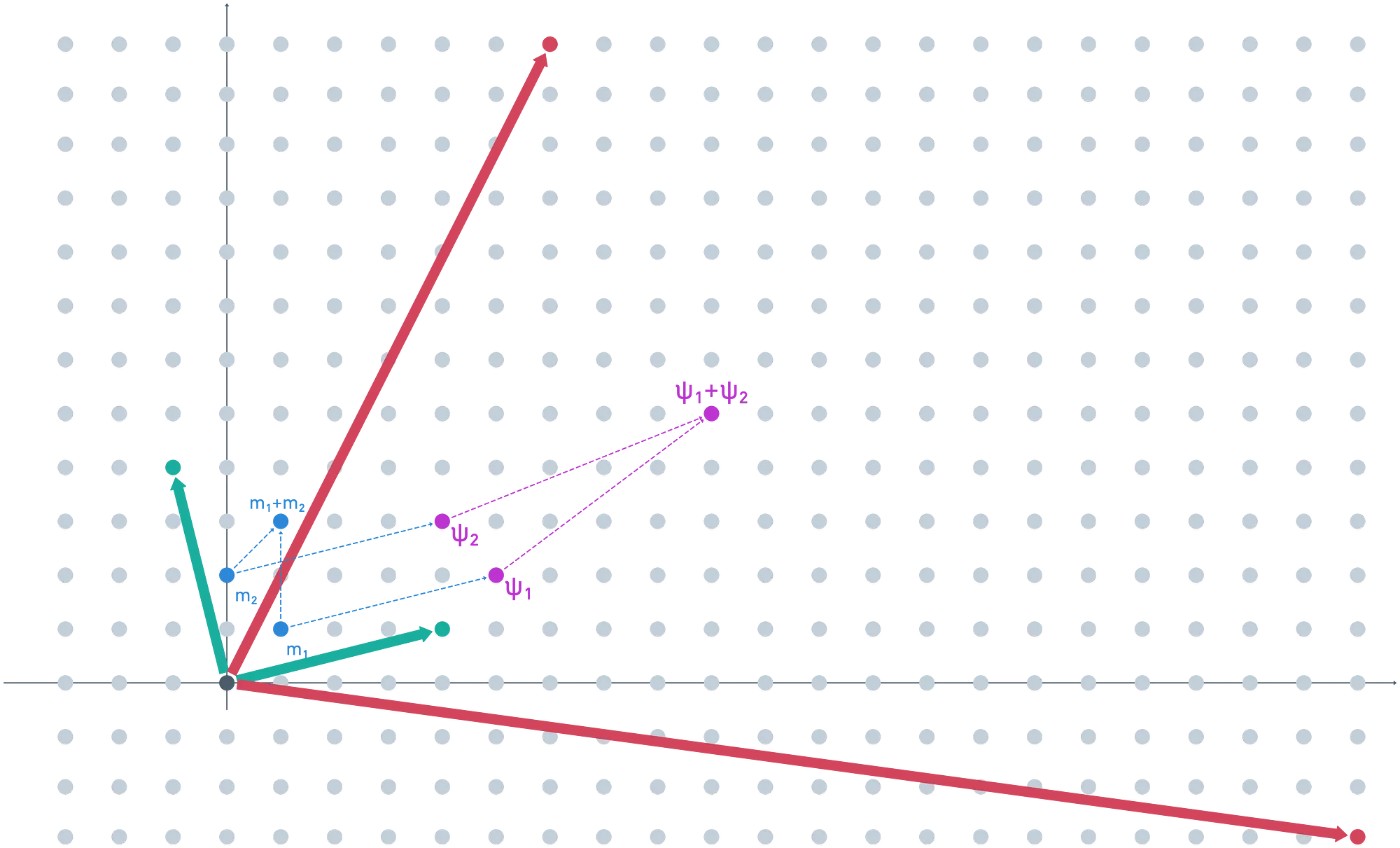
Suppose $m_1 = (1,1)$, $m_2 = (0,2)$. Of course, when added, these should yield $(1,3)$. We expect our scheme to return this value upon decryption.

After adding some small noise, we obtain our ciphertexts, which result in the vectors $\psi_1 = (5,2)$ and $\psi_2 = (4,3)$. We should be able to add them, and the result should decrypt to $m_1 + m_2$.

Click to zoom

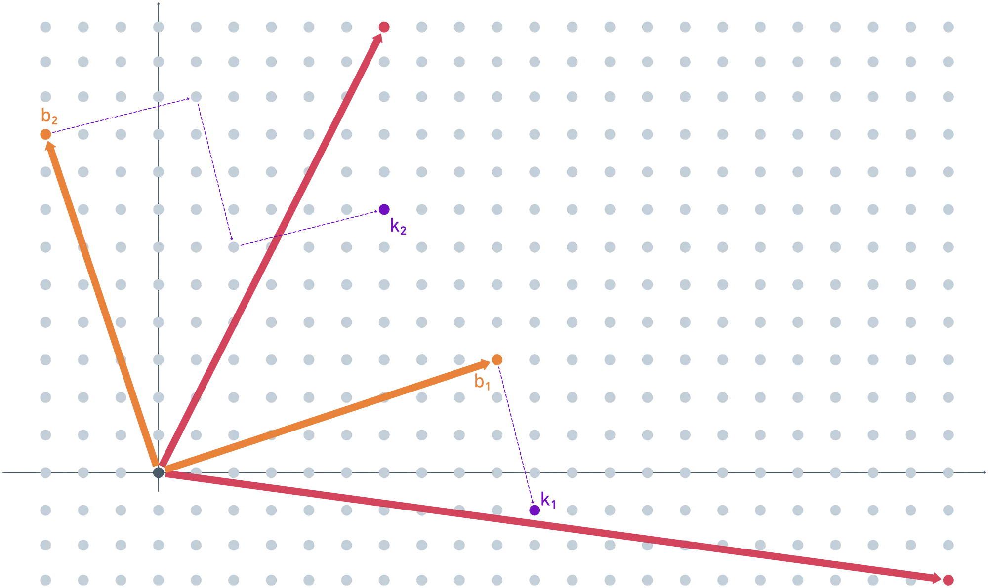
Onto the fun part now. We need to encrypt the secret key, so we add some noise $i$ to each vector (it doesn’t have to be the same value as before), and map the results modulo the public key. We get $k_1 = (10, -1)$ and $k_2 = (6,7)$ as the encrypted values for the secret key.

For simplicity, I chose appropriate noises so that the results were already part of the fundamental parallelepiped of the public key.

Click to zoom

Next up, we want to perform this homomorphic decryption stuff. The idea is to map the ciphertext to the domain of the secret key, but encrypted. Doing this yields $(12,1)$ — our refreshed ciphertext!

Click to zoom

All that remains is checking that this decrypts to the correct value. We do this just as before — take $\textrm{mod}$ the secret key (unencrypted), and then mod our plaintext domain, $I$.

Click to zoom

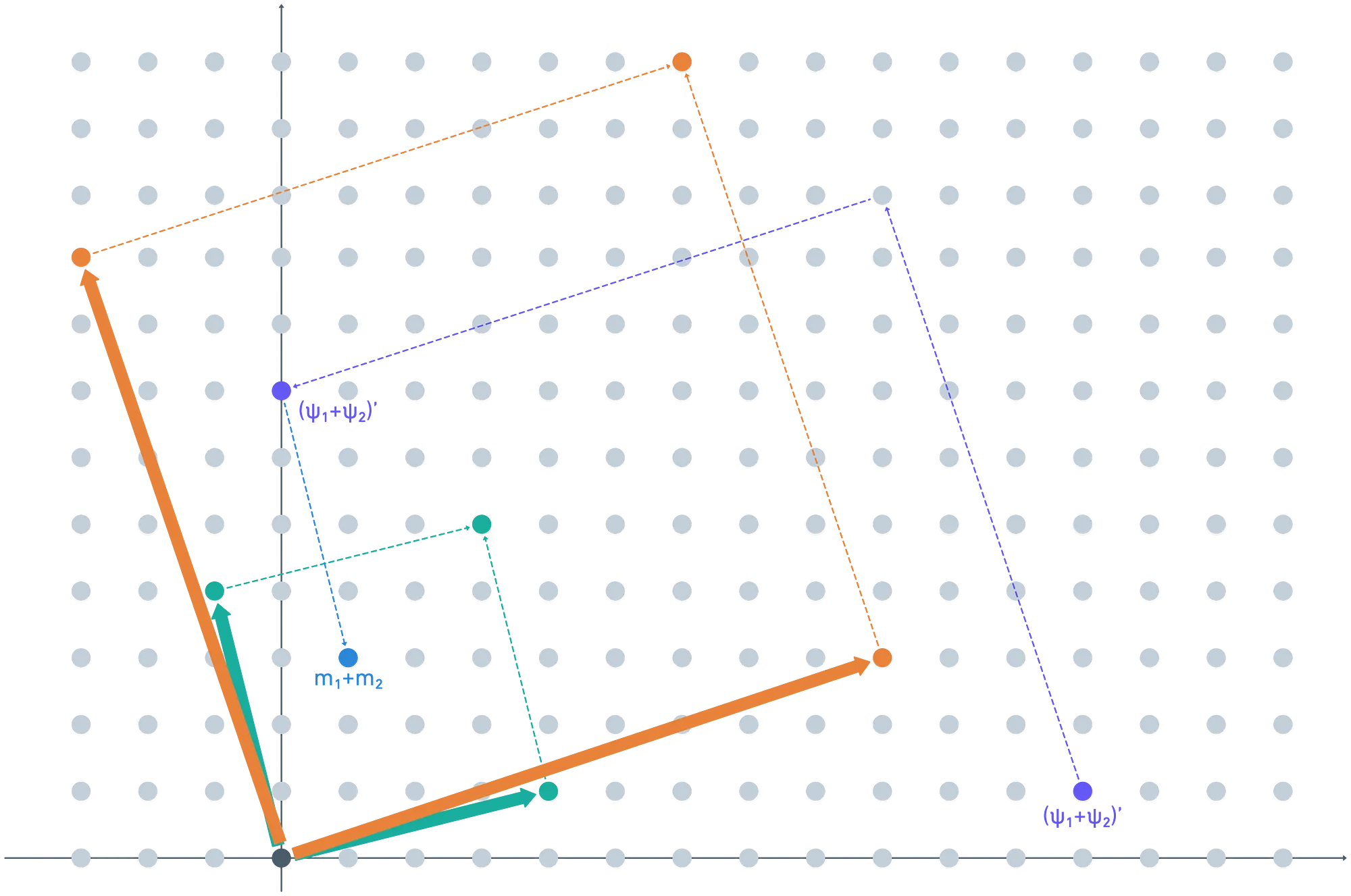
Just like clockwork, we get back the correct value $(1,3)$!

But what happened to the noises during this entire ordeal?

Noise in this context is expressed as the smallest linear combination of $B_I$ vectors that results in a point in the same coset (in $J$) as our ciphertext. For the refreshed ciphertext, it’s easy to see that the difference is quite small (a single vector in our basis).

Finding the representative for the original $\psi_1 + \psi_2$ is not as simple, though. Here, I’ll show you where the cosets match:

Click to zoom

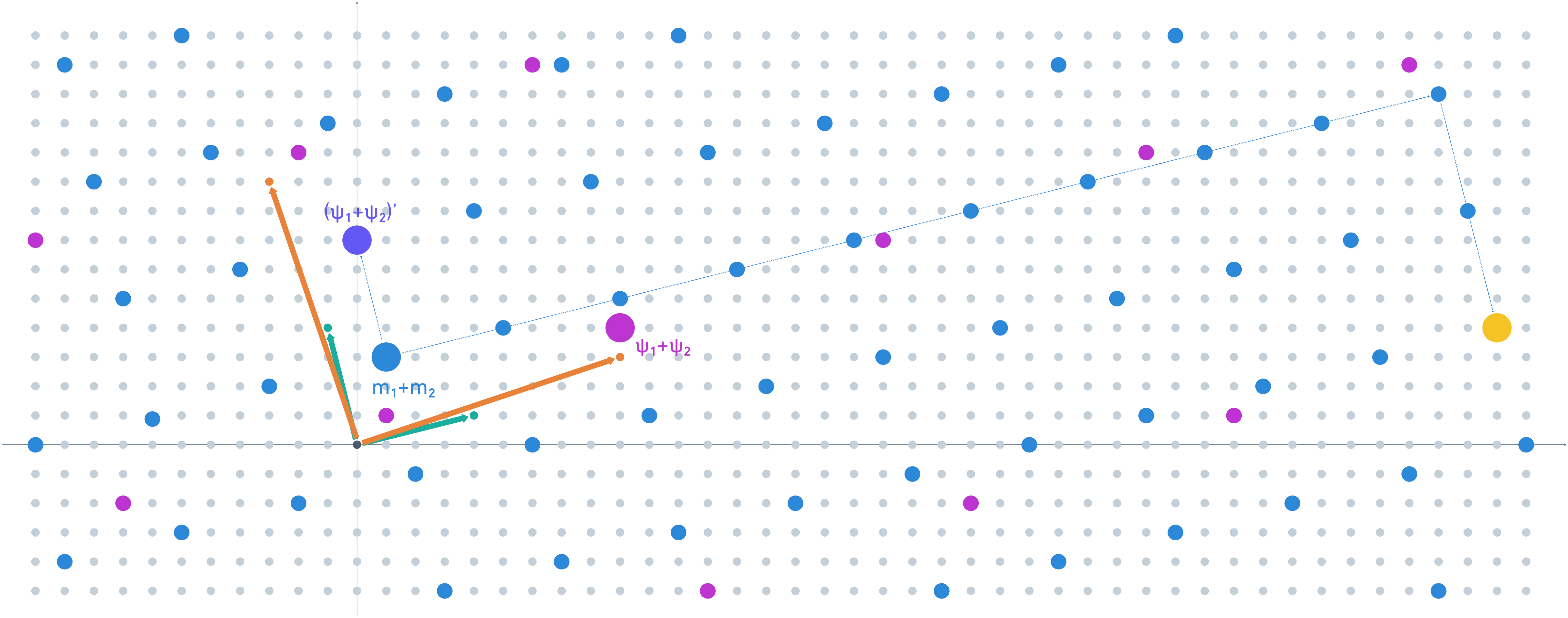
Admittedly, this error growth relates to a poor initial choice of $J$.

In Gentry’s construction, the vectors in the secret key ($R/J$) are tens or hundreds of times bigger than the basis vectors for $R/I$. Our scenario doesn’t quiet comply with these terms — because I couldn’t possibly fit all those points into a single screen!

But hey, at least it helps illustrate how the bootstrapping process works. A pretty large portion of the noise was reduced very effectively!

Summary

Of course, the story doesn’t end here. As it stands, this algorithm is very impractical. The original paper (and the thesis, which is a bit more friendly to read) actually introduces some improvements for the algorithm to be practical, but we won’t get into that.

What’s important is that this work proved that FHE was possible. The code had been cracked, and something that was seemingly unachievable was made possible.

Nowadays, there are newer and shinier techniques that improve on Gentry’s original work (after all, it was published 15 years ago). For example, there’s this 2011 paper where another method for FHE without bootstrapping is proposed. Or this 2014 paper, which describes a much faster FHE method.

Spoiler: it doesn’t get any easier than this article here!

The field has evolved quite a lot, so I’d like you to think of this text as a short primer on the topic!

And if you need FHE implemented in a project, there are lots of libraries out there for this purpose.

Closing Words

What a ride it has been!

Even though I’ve learned a lot during the making of this series, I’ll say the exact same thing I said at the very beginning: I’m still not an expert in the subject — just a guy trying to learn the craft on his own.

And who is maybe a tad more knowledgable!

Still, I believe this journey was deeply enriching.

The sheer amount of information and tools available nowadays is simply astounding. It’s easier than ever to learn stuff.

But sometimes, it’s hard not to go down unending rabbit holes, or not to get tangled up in the weeds — especially when dealing with highly-specialized topics. My aim was to simplify a bit, and make things a little more digestible.

I wholeheartedly hope this series has hit the mark in helping someone better understand the very complex concepts that cryptography has to offer. And I hope you had a laugh or two along the way. For me at least, it has been super fun.

Hope to see you around soon! And stay tuned for more content!