Arkana | Cryptography 101: Pairings

This is part of a larger series of articles about cryptography. If this is the first article you come across, I strongly recommend starting from the beginning of the series.

We've already explored several applications for elliptic curves — some simple schemes and some more advanced ones. We also threw polynomials into the mix when studying threshold signatures. If we stretch the limits of creativity, we can still devise a lot of protocols based solely on these constructions.

But this doesn't mean that there aren't other tools out there. And there's a very important one that we still need to present: pairings.

In this article, we'll define what they are — but not how to compute them. The reason for this is that we haven't yet defined the mathematical machinery needed for pairing computation. This, we may explore at a later time, but if you're interested, this is an excellent resource to look at in the meanwhile. And there are also lots of libraries out there that cover pairing computation if you want to start fiddling with them after reading this article!

•••

Pairings

A pairing, also referred to as a bilinear map, is really just a function, typically represented with the letter $e$ . It takes two arguments, and produces a single output, like this:

e: \mathbb{G}_1 \times \mathbb{G}_2 \rightarrow \mathbb{G}_3 \ / \ e(G_1, G_2) = G_3

We'll require some notation from set theory this time around, but nothing too crazy.

Probably the most exotic one (if you haven't had much prior contact with set theory) is the cartesian product — used in the set $\mathbb{G}_1 \times \mathbb{G}_2$ . It's just the set of all elements of the form $(G_1, G_2)$ where $G_1$ belongs to $\mathbb{G}_1$ , and $G_2$ belongs to $\mathbb{G}_2$ .

However, this is not any ordinary function. It has an important property: it is linear in both inputs. This means that all of the following are equivalent:

e([a]G_1, [b]G_2) = e(G_1, [b]G_2)^a = e(G_1, G_2)^ab = e([b]G_1, [a]G_2)

As you can see, we can do this kind of switcheroo of the products (or more precisely, group operations). Even though this property doesn't amount to much at first glance, it's really very powerful.

Pairings are a sort of blender, in the sense that we don't really care that much about the particular value obtained when evaluating a pairing expression (except when checking something called non-degeneracy). Instead, what we care about is that some combinations of inputs yield the same result, because of the bilinearity we mentioned above. This is what makes them attractive, as we'll see further ahead.

Elliptic Curves and Pairings

Notice how the inputs come from the cartesian product $\mathbb{G}_1 \times \mathbb{G}_2$ . It's a rather particular set: $\mathbb{G}_1$ and $\mathbb{G}_2$ are groups, to be precise. Disjoint groups, in fact — meaning that they don't share any elements. Formally, we say that their intersection is empty:

\mathbb{G}_1 \cap \mathbb{G}_2 = \varnothing

In addition, $\mathbb{G}_1$ and $\mathbb{G}_2$ aren't just any groups — they must be suitable for pairing computation. Turns out elliptic curve groups happen to be a good choice — and a very good one in terms of computational efficiency. So it's a happy coincidence that we already have a good grasp on them!

If you check the literature, there are instances where instead of using two disjoint groups, you'll see the same group being used twice. Something like $\mathbb{G} \times \mathbb{G}$ .

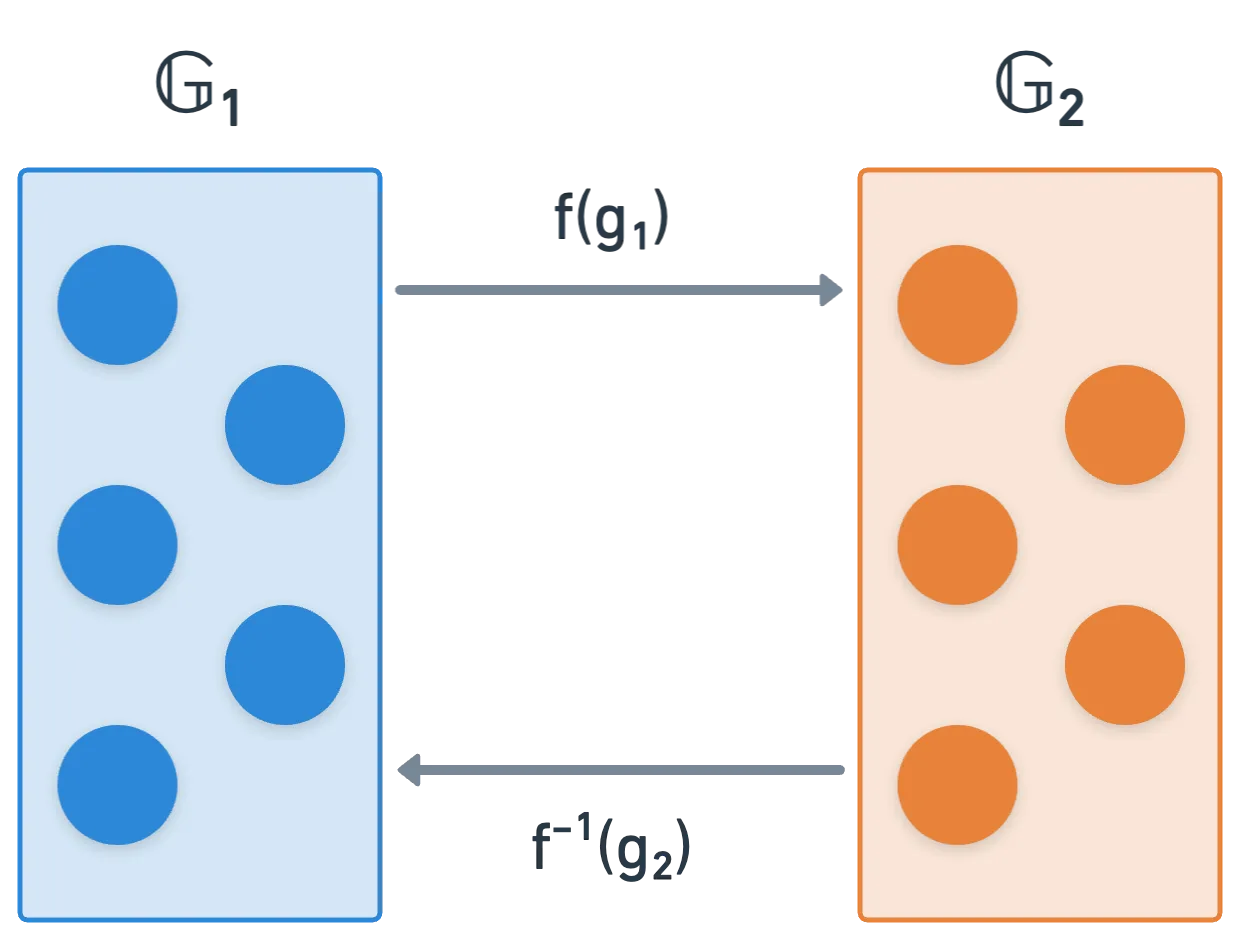
These are sometimes called self-pairings, and what really happens is that there's a function f that maps $\mathbb{G}_2$ into $\mathbb{G}$ — meaning that we can transform elements of $\mathbb{G}_2$ into elements of $\mathbb{G}$ , and just use $\mathbb{G}$ in our pairing.

Even though we'll not cover how this is done, bear in mind that the formal definition of a pairing requires the groups to be disjoint.

Visualization of the sets in a pairing — Some function f allows moving back and forth from the groups G₁ and G₂.

•••

Application

Before we get to the point of "why the hell am I learning this" (assuming we're not there yet!), I believe it fruitful to present an application.

Despite the fact that we don't know how to compute pairings yet, we can understand their usefulness because we know about their properties.

Let's waste no time and get right to it.

The Setup

Working with elliptic curve groups, or even with integers modulo $p$ , can get you really far. But you know one thing neither of them can do for you? They don't allow you to use your identity for cryptographic operations!

Bryan Cranston dropping the mic — Boom! Mic drop!

Identity? You mean like my name? Sounds bonkers, but it can be done. Some setup is required, though.

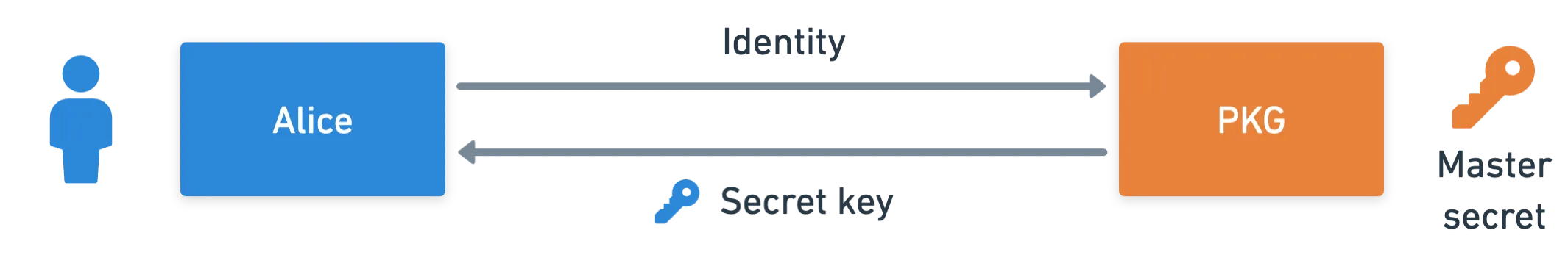
To perform this kind of cryptographic magic feat, we'll need a special actor, trusted by other parties — often referred to as a Trusted Authority. This actor will be in charge of private key generation, so it's also accurately (and very descriptively) named a Private Key Generator (PKG).

The PKG does a few things. First and most importantly, they choose a master secret, which is an integer $s$ . They also choose and make public some public parameters, which we'll define in a minute. And finally, they choose and make public a hashing function $H$ , which hashes into $\mathbb{G}_1$ .

H: \{0,1\}^* \rightarrow \mathbb{G}_1

To get ahold of a private key, Alice has to request it from the PKG. And to do so, she sends them her hashed identity. Her identity could be anything — a name, an email address, an identity document number, anything that uniquely identifies an individual. We'll denote this as $ID$ . Her public key is then:

Q_A = H(ID_A) \in \mathbb{G}_1

Upon receiving this value, the PKG calculates her private key as:

S_A = [s]Q_A \in \mathbb{G}_1

And sends it to Alice.

All of these communications are assumed to happen over a secure channel. In particular, Alice's secret key should not be leaked!

Our setup is done! Alice has both her private and public key. What can she do with this?

Identity-Based Encryption

Let's suppose Alice wants to encrypt a message for Bob. All she has is his public key, because she knows his identity ( $ID$ ). And just by hashing it, she obtains his public key:

Q_B = H(ID_B)

We're also going to need a couple more things:

A point $P \in \mathbb{G}_2$ , used to calculate a point $Q = [s]P$ , also in $\mathbb{G}_2$ . Since $s$ is only known to the trusted authority, these points are calculated and published by the PKG — they are the public parameters we mentioned earlier, and we'll denote them by $p$ :

p = (P, Q)

We also need another hash function $H'$ :

H': \mathbb{G}_3 \rightarrow \{0,1\}^n

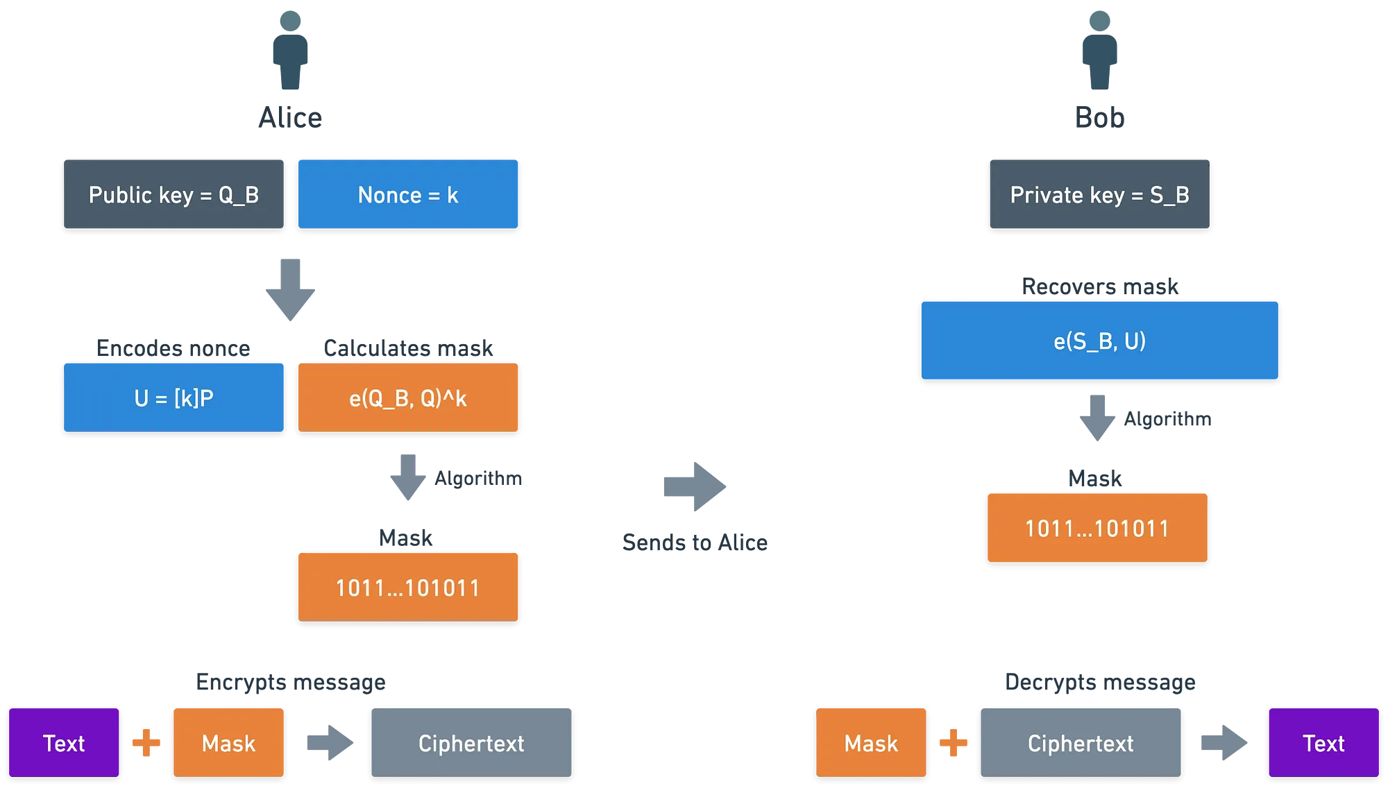
This encryption scheme uses a similar strategy to the Elliptic Curve Integrated Encryption Scheme we saw earlier in the series: masking. So in order to encrypt a message $M$ , Alice follows these steps:

She chooses a random nonce, which is an integer $k$ .
With it, she calculates $U = [k]P$ . This will be used to later reconstruct the mask.
Then, using Bob's public key, which is just the hash of his identity, she computes:

e(Q_B,Q)^k

She uses this value to compute a mask, which is added to the message:

V = M \oplus H'(e(Q_B,Q)^k)

The final encrypted message will be the tuple $(U, V)$ .

Remember that the $\oplus$ symbol represents the XOR operation. And one of the properties of this operation is: $M \oplus A \oplus A = M$ . What this means is that adding the mask twice allows us to recover the original message.

How does Bob decrypt? Well, he can take $U$ and simply recalculate the mask. With it, he re-obtains the original message:

M = V \oplus H'(e(S_B,U))

But wait... How are the two masks equal to each other? Clearly, they don't look like the same thing... They are different evaluations of the pairing!

e(Q_B,Q)^k \stackrel{?}{=} e(S_B,U)

Fear not — I promise this makes sense. Because this is precisely where the magic of pairings happens: using their bilinearity property, we can show that the two values are equivalent:

e(Q_B,Q)^k = e(Q_B, [s]P)^k = e(Q_B, P)^{s.k} = e([s]Q_B, [k]P)

e(Q_B,Q)^k = e(S_B, U)

And just like that, knowing only Bob's identity is enough for Alice to encrypt information just for him — powered by pairings, of course!

Diagram of encryption using pairings — To summarize, here's a visual representation of the process

•••

Back to Pairings

Okay, now that we've seen pairings in action, we're fully motivated to understand how they are defined a bit more in-depth. Right? Right?

Jurassic Park T-Rex scene — Oh I can see you there

This won't take too long—we'll just take a quick peek at some of the ideas that make pairings possible.

We mentioned that $\mathbb{G}_1$ and $\mathbb{G}_2$ could very well be elliptic curve groups.

So, do we just choose two different elliptic curves? Well, in that case, we would have to make sure the groups are disjoint, which is not necessarily easy; and there are other concerns in such a scenario.

What about using a single elliptic curve? Then we would need two different subgroups. When we make use of a group generator, $G$ , the group generated by it is not necessarily the entirety of the elliptic curve group — but it could be. This inclusion relation is written as:

\langle G \rangle \subseteq E(\mathbb{F}_q)

Which means: the group generated by $G$ is either a subgroup, or the entire elliptic curve.

We usually want the order of the subgroup generated by $G$ to be as large as possible, so that the DLP problem is hard. This means that:

If there are other subgroups, they are probably small.
If $\langle G \rangle$ is the entirety of the elliptic curve, then there are no other available subgroups.

We seem to have reached a conundrum...

Finding Nemo scene of fishes in bags — What now, chief?

Expanding the Curve

Luckily, this little crisis of ours has a solution. You see, our curves have been always been defined over the integers modulo $q$ — but what if we could extend the possible values that we use?

Instead of only allowing the points in the elliptic curve to take values in the integers modulo $q$ :

\mathbb{F}_q = \{0,1,2,3,..., q-1\}

We could use something like the complex numbers, and allow the points in $E$ to take values in this set:

\mathbb{F}_{q^2} = \{a + bi : a, b \in \mathbb{F}_q, i^2 + 1 = 0 \}

Using complex numbers makes perfect sense: for example, you can check for yourself that the point $(8, i)$ lies on the following elliptic curve:

E/\mathbb{F}_{11}: y^2 = x^3 + 4

Field Extensions

Complex numbers are just one example of a more general concept, which is field extensions.

A field (we'll denote it $F$ ) is just a set with some associated operations. This probably rings a bell — it's a very similar definition to the one we gave for groups, at the very start of the series.

Regardless of the formality, there's a very important field we should care about: the integers modulo $q$ , when $q$ is a prime number.

This may sound a bit misleading. Originally, I told you the integers modulo $q$ were a group. And indeed, if we use a single operation (like addition), they behave like a group.

More generally though, they are a field, as they support addition, subtraction, multiplication, and division (well, modular inverses, really!).

A field extension is simply a set $K$ that contains the original field:

F \subset K

Under the condition that the result of operations between elements of $F$ always lie in $F$ , but never in the rest of $K$ (the set $K - F$ ).

One very well known field extension is of course the set of the complex numbers. The real numbers act as $F$ , and operations between real numbers (addition, subtraction, multiplication, and division) lie in the real numbers ( $F$ ) as well. Operations between complex numbers may or may not result in real numbers.

Why does this matter? Imagine we define a curve over the integers modulo $q$ . We get a bunch of points, which we can denote:

E(F)

If we extend the base field (the integers modulo $q$ ), then new valid points will appear, while preserving the old ones. This is:

E(F) \subseteq E(K)

Because of this, new subgroups appear, and we get the added bonus of keeping the original subgroups, which were defined over the base field.

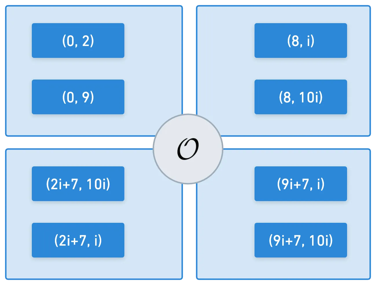
And when we choose an appropriate field extension, something amazing happens: we get a plethora of subgroups with the same order as $\langle G \rangle$ . And these groups happen to be almost disjoint: they only share the identity element, $\mathcal{O}$ . The set of all these subgroups is what's called the torsion group.

Torsion group representation — 3-torsion group of the curve E/F₁₁: y² = x³ + 4. Each blue box is a subgroup, along with 𝒪, which is common to all subgroups — hence it's depiction in the center.

•••

Okay, let's stop there. The goal of this section is just to present a general idea of what pairing inputs are. However, there's not much more we can say without taking a deeper dive into the subject, which is something that exceeds the scope of this introductory article.

Again, I recommend this book if you want a more detailed explanation — and in turn, it references some great more advanced resources.

The important idea here is that pairing computation is not trivial, by any means. If you're interested in me expanding topic further in following articles, please let me know!

•••

Summary

Even though we haven't ventured deep into the territory of pairings, this simple introduction allows us to understand the working principle behind pairing-based methods. Everything hinges on the bilinearity property that we saw right at the beginning of the article.

The key takeaway here is:

Pairings are these sort of blenders, where we care about the computed result being the same for two different sets of inputs

Again, we might dive into pairing computation later on. I believe it to be more fruitful to start seeing some applications instead.

For this reason, we'll be looking at a couple more pairing applications in the next installment in the series. See you then!