Elliptic Curves In-Depth (Part 2)

Last time around, we defined what elliptic curves are, and we devised a (suspiciously convoluted) way to add points on the curve together. And we hinted at how this operation was key for cryptographic applications.

However, the curves themselves — defined over the real numbers — are not the constructions we’re after.

Cryptography is a discipline of discrete precision. We want algorithms that yield consistent, reproducible results. In other words, we’re after determinism, which roughly speaking means that using the same inputs should yield the same outputs, no matter what.

Working with real numbers is quite cumbersome in this sense, because we normally use floating point arithmetic, and consequently, rounding errors are always present, making operations imprecise.

Due to rounding errors, the result of adding $P \oplus Q$ may not even land exactly on the curve (when working over the real numbers).

This calls for a different strategy.

That will be our starting point for today! We’ll kick things off with a minor detour, and then come right back to elliptic curves.

A Suitable Domain

As opposed to the real numbers, the integers are very precise to operate with. Since there are no decimals to worry about, rounding errors seem to be off the menu!

While this is true for addition, subtraction, and multiplication, it looks like division might be a bit of a problem: $1$ divided by $3$ clearly does not yield an integer, and we’re back in the realm of floating point arithmetic.

It’s also worth asking ourselves how large we can allow our integers to be. After all, we need to represent them somehow — and allowing them to grow too large is problematic when trying to store and handle them in a computer.

So yeah, integers — and more specifically, positive integers — , but we’re halfway there. We need a way to keep our values in check (bounded), while also figuring out how to handle division.

Modular Arithmetic

To remediate this, we’ll make use of a simple tool: the modulo operation, and modular arithmetic.

I’ve talked about this in previous articles, so I’ll assume familiarity with these concepts.

By using the modulo operation to bound results from our addition, subtraction, and multiplication operations, we essentially limit the possible integers we can work with to a finite set, such as this one:

$$\mathbb{F}_{11} = \{0,1,2,3,4,5,6,7,8,9,10\}$$

We’re using the symbol $\mathbb{F}$ here, because the resulting set will be a field (hence the $\mathbb{F}$). A field is just a set where addition, subtraction, multiplication, and division are well-defined.

That’s one problem down (boundedness). Since our field is now a finite set, we just call it a finite field.

Division will require some more work — along with a clever observation.

A Different View

Take for example $5 \ \textrm{mod} \ 3$. Obviously the result is $2$. How did we get there?

We can more rigorously describe the process as finding a solution to this equation:

$$5 = 3k + x$$

And requiring $x$ to be a value between $0$ and $4$ (an element of $\mathbb{F}_5$). This results in $k = 1$ and $x = 2$.

It’s clear, however, that other solutions exist. For example, $k = 2$ and $x = -1$. As you can probably tell by now, we can find infinitely many integer solutions to this equation.

In fact, the set of all possible values for $x$ forms an equivalence class.

Yeah ok... Why should we care? Turns out that by looking at it this way, there’s something we can do about division!

If we really think about it, the result of some division $1 / a$ is nothing more than another number, which satisfies a particular property. For instance, the result of $1 / 2$ is $0.5$, and for $1 / 3$, we get $0.333(...)$. These results all share this property:

$$a.\left ( \frac{1}{a} \right) = 1$$

So, instead of thinking in terms of division, let’s think of it in terms of finding a reciprocal number. We ask ourselves:

Given some number in our field, can we find another number (also in the field), so that when we multiply them together, the result is $1$?

In other words, we’re after a solution to this equation:

$$a.x \ \textrm{mod} \ p = 1$$

Which — you probably guessed it — can be translated into this form:

$$a.x - p.k = 1$$

And we’re back in the scenario from before! If we happen to be able to find a valid value for $x$, we say it’s the modular inverse of $a$, and we write it as $a^{-1}$.

This form is known as Bézout’s identity, and we of course only care about integer solutions for $x$ and $k$ (it’s a linear Diophantine equation).

Importantly, a solution might not exist. Excluding zero, the condition for the modular inverse of an integer $a$ to exist is that it’s coprime with the field size $p$, meaning that they share no factors — or that their greatest common divisor (GCD) is $1$.

We can prove this very quickly. Suppose $a$ and $p$ share some factor $t$, meaning that $a = t.a’$ and $p = t.p’$. Then, we could factor $t$ out, and the above equation would become:

$$t(a'.x - k.p') = 1$$

No matter what values of $x$ and $k$ we use, the left-hand side will never be $1$, meaning that the equation would have no solution. Consequently, if a and $p$ share $a$ factor, then the modular inverse doesn’t exist.

There’s a very simple workaround for this: choosing a prime number for $p$! By definition, any prime number has only two factors: $1$, and itself — meaning that, as long as the finite field has a prime size, then all of its elements (excluding zero) will have a modular inverse.

Well, in fact, by definition, the inverse of $0$ is $0$.

Awesome stuff! This means that something akin to division is defined for every element in the set — it’s indeed a field.

Back to Elliptic Curves

Operations between elements of a finite field yield deterministic and well-defined results, which is exactly what we wanted!

Now all we need is to define our elliptic curves over these sets, instead of over the real numbers. There’s nothing too fancy going on here — we have already derived explicit formulas for point addition and doubling in our previous encounter. The only tweak we must do is to replace division with multiplication by modular inverses.

For example, point doubling is done by simply running these calculations below:

$$\\ m = (3x_P + a)(2y_P)^{-1} \\ n = y_P - mx_P$$ $$\\ x_R = m^2 - 2x_P \\ y_R = -(mx_R + n)$$

So yeah, nothing fancy — except that all those results are taken modulo $p$. We also know that they are elements in our finite field — meaning that the resulting $R$ will have integer coordinates as well.

There’s a subtlety to be noted here. When we analyzed the case in the real numbers, we were guaranteed to find a third intersection point. It’s not immediately obvious that this translates to a finite field setting. Luckily for us, adding and doubling operations are also pretty well-behaved on finite fields!

Because of this, elliptic curves will not look like “curves” per se when defined over finite fields. Instead, they will look more like a set of points bounded to a square of side length $p$, like this:

Click to zoom

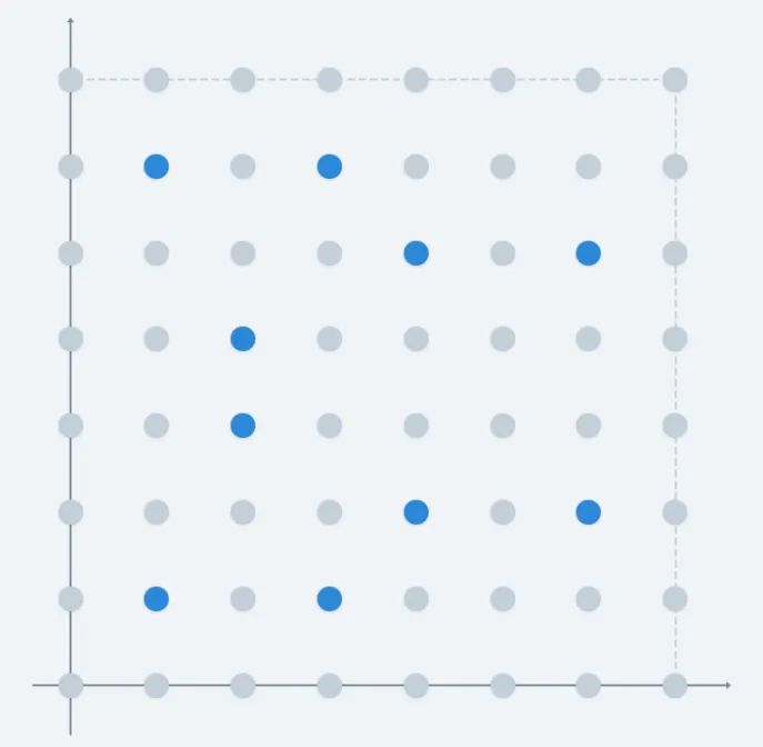
You can play around with different curves here.

And of course, we're not counting the point at infinity!

It’s not evident just by looking at this picture what the result of adding any two points on the curve is. Still, the chord and tangent rules are defined by the equations we already derived, regardless of the fact that we’re working with a different set. It’s just that visuals don’t help much now:

Click to zoom

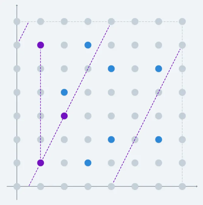
As you can see, the lines get cut when they reach the boundaries of our square domain — and this makes sense, because the lines are also defined modulo $p$.

Everything is defined modulo $p$ now!

A more natural way to think about this, is by noting that the left and right borders are equivalent under modulo $7$ ($7 \ \textrm{mod} \ 7 = 0$), so if we could bend our square into three dimensions, we could paste those edges together, getting a 3D cylindric surface. Let’s explore this, just for fun.

The same can be done with the top and bottom edges. It takes a bit of imagination, but it’s as if our elliptic curve is really defined over a doughnut-shaped domain — a torus. In that space, the lines would effectively be continuous!

Click to zoom

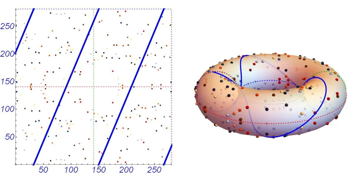
For those out there who have studied topology, this will be very reminiscent of quotient topologies!

We need not care for these transformations, but it’s always a good exercise to try and push our understanding a bit further, as it may help gain new insights.

Speaking of which — there’s a particularly pesky point we haven’t dealt with very gracefully so far: the point at infinity. It feels a bit forced — we can’t seem to place it anywhere. And after our little exercise with bending and doughnuts, let’s see if we can find a way to place it somewhere.

Projective Coordinates

Since our curve is defined over either $\mathbb{R}^2$ or ${\mathbb{F}_p}^2$, it’s not crazy that we’ve pictured elliptic curves as points on a plane (or a deformed plane, in the cases we examined just moments ago).

This is called affine space (together with the point at infinity), sometimes denoted $\mathbb{A}^2$.

Here’s a rather unusual question: where can we place that plane? I mean, a plane is just a plane — an abstract canvas for us to represent things on. Does it even make sense to try to place it somewhere?

As a matter of fact, yes! And the first step to do so, is to move one dimension up.

In three dimensions, a plane is actually defined by a linear equation:

$$p: ax + by + cz + d = 0$$

There are infinitely many different planes we could represent in three dimensions. Now “placing” a plane somewhere does make sense—all we need is to choose one of the infinitely many planes that are available for us in 3D space.

And we don’t need anything fancy, really. We can just choose the horizontal ($x-y$) plane that sits at $z = 1$. Imagine we draw our elliptic curve on this plane.

Here’s where it gets interesting: for each point $P=(x,y)$ on the curve, if we draw a line passing through the origin $(0,0,0)$ and $(x,y,1)$, that line will intersect the plane $z = 1$ at exactly one point: $P$. So these lines are equivalent to the point themselves!

Click to zoom

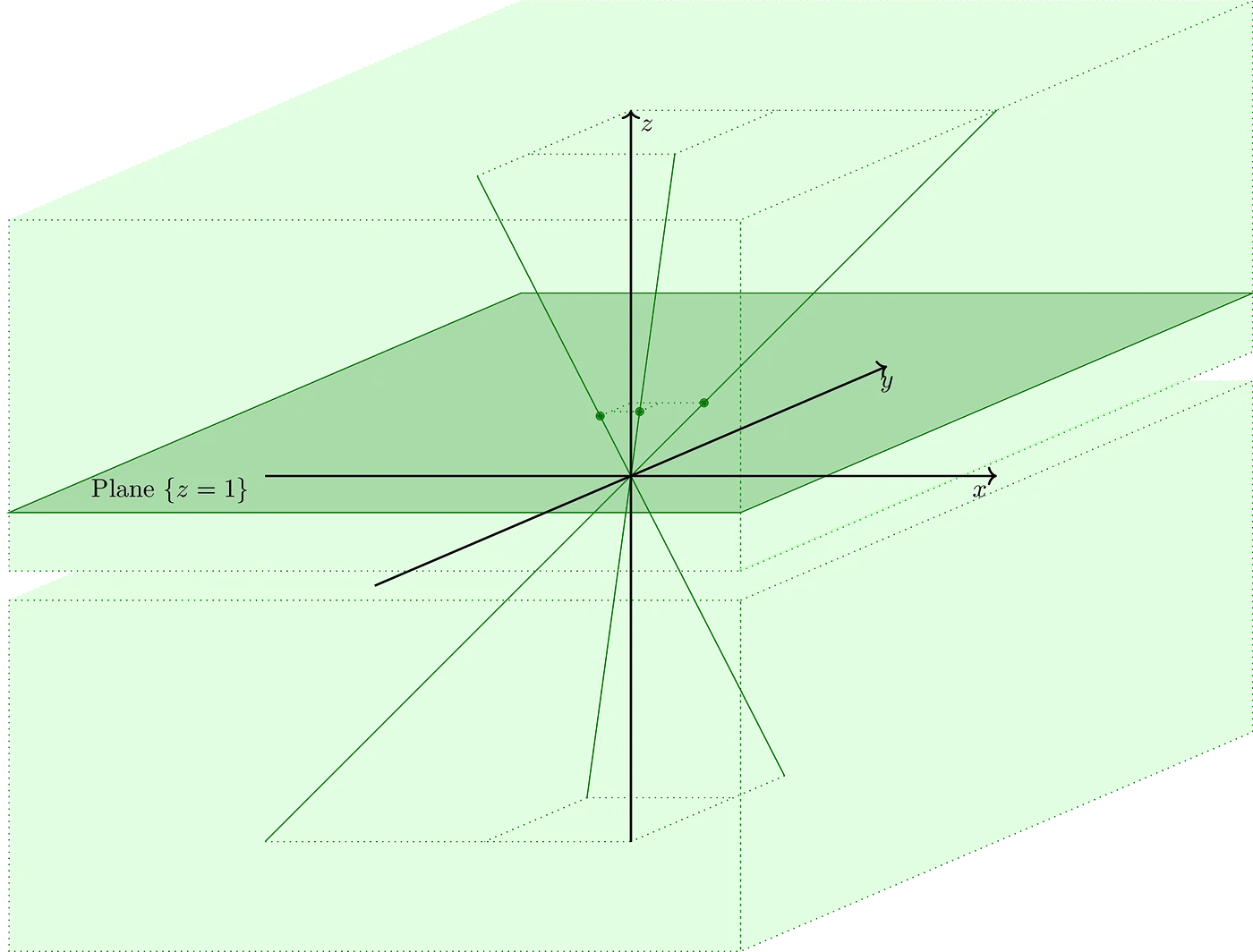
This is called projective space, and is denoted by $\mathbb{P}^2$. To make things a bit clearer, let’s denote points in this 3D space by $(X,Y,Z)$.

Now, any point in any of these lines preserves the ratio $X:Y:Z$. This is, if we examine the line defined by $P=(x,y,1)$, then the point $(2x,2y,2)$ will lie on the same line, and so will $(3x, 3y, 3)$, or generally speaking, any point of the form $(tx, ty, t)$. This is usually represented via the notation $(X:Y:Z)$ to reflect this notion of ratios.

Because we chose $z = 1$, we can recover the original $x$ and $y$ values via:

$$x = X / Z, y = Y / Z$$

And these expressions can be substituted into our elliptic curve equation, yielding this expression:

$$e: \frac{Y^2}{Z^2} = \frac{X^3}{Z^3} + a\frac{X}{Z} + b$$

Which, after clearing the denominators, yields:

$$e: Y^2Z = X^3 + aXZ^2 + bZ^3$$

Let’s take a breather for a second. I must admit: this smells like an unnecessary complication.

But sometimes, these seemingly unnecessary complications can reveal new insights that may make our lives much easier.

Here’s a great video that perfectly illustrates this idea. It doesn’t have much to do with elliptic curves, but I think it’s simply amazing!

Upon closer inspection, something fantastic has happened indeed.

You see, every point on the curve that lives on the plane $z = 1$ has the form $(X,Y,1)$. However, a “point on the curve” is really any point that satisfies the equation $e$. There’s no real reason to restrict ourselves to a plane here.

Yet, we’re working with these projective coordinates — where each line starting at the origin is an equivalence class. And in this setting, there happens to be another point that satisfies the equation: the point $(0,1,0)$. You can check this yourself — it just works!

This line is completely parallel to the plane $z = 1$ — so it never intersects it. It satisfies the equation, yet it has no representative point in our affine space (the plane).

Sounds familiar?

Guess what — this is the point at infinity we’re looking for, but we can actually represent it now! Showing this fact takes a little effort, though. In the interest of not overcomplicating things, we’ll avoid going down that path.

Usefulness

Projective coordinates offer this new visibility over the point at infinity. Naturally, we may wonder if that’s all they are good for, or if it’s just an extremely contrived artifact to gain some additional understanding.

As it turns out, projective coordinates are quite useful! When we work out the formulas for point addition and multiplication, something interesting happens: we’re able to avoid some modular inverses!

Modular inverses are quite expensive to calculate. The standard algorithm to calculate them is the Extended Euclidean algorithm.

We’ll not be covering it here for the sake of brevity, but you can see how it works here.

What’s for sure is that it takes considerably more effort than simple multiplications. And so, using projective coordinates leads to faster elliptic curve operations!

In cryptography, where we need to perform thousands or millions of these operations, every little bit counts.

Summary

We’ve covered quite a bit of ground today! We moved from real numbers to finite fields, saw how our curves transform in this new setting, and even found a way to properly represent our point at infinity.

Of course, this is far from being the end of the story.

We have yet to talk about what makes elliptic curves useful in cryptography. But now that we’re working in this bounded setting, something remarkable happens: elliptic curves behave like groups. This is what gives them their cryptographic superpowers.

Next time, we’ll explore this group structure, see why it’s useful, and finally get to the heart of why elliptic curves are such a fundamental tool in modern cryptography.

Until then!