Cryptography 101: Zero Knowledge Proofs (Part 2)
This is part of a larger series of articles about cryptography. If this is the first article you come across, I strongly recommend starting from the beginning of the series.
In the past few articles, we've covered a lot of building blocks. It's time to finally combine all these lego pieces into a protocol. Hooray!
Remember, the reason we made such an effort to understand these moving parts was to try and build a general framework for zero knowledge proofs — because, as we saw, creating a protocol for a specific application was somewhat impractical, requiring specific research.
We're now ready to introduce a family of knowledge proofs that utilizes every element we've preemptively defined: SNARKs.
Specifically, we'll be looking at a scheme called Plonk. For a full disclosure of the technique, go here. I'll try my best to explain this as precisely as possible. Moreover, this is not the only protocol that qualifies as a SNARK out there. Other mechanisms such as Groth16, Marlin, and Halo exist. I might tackle those in the future, but for now, I'll just leave a couple links here in case you want to follow your curiosity!
Disclaimer
This article is gonna be long, and honestly, complex. As in, probably harder than usual. There's only so much I can do to simplify the explanation for a protocol that is pretty darn complex.
But, if I had to put this entire process into a single phrase, it would be:
![]()
![]() In Plonk, we encode the computation of a circuit into a series of polynomials, which represent the constraints imposed by the circuit, for which we can prove statements by using a series of tests, without ever revealing the polynomials themselves — and thus, not leaking the secret inputs.
In Plonk, we encode the computation of a circuit into a series of polynomials, which represent the constraints imposed by the circuit, for which we can prove statements by using a series of tests, without ever revealing the polynomials themselves — and thus, not leaking the secret inputs.![]()
![]()
Getting to fully understand this will be a wild ride. And there are several elements that we'll need to cover. Here's an overview of the plan, which doubles up as a sort of table of contents:
- Circuits as sets of constraints
- Encoding the circuit into polynomials
- Listing the requirements for verification
- Techniques for verification
- Verification
Also, I'm assuming you already checked out the article about polynomial commitment schemes, and also the one about arithmetic circuits. If you haven't, I strongly recommend reading them!
Without further ado, here we go!
What is a SNARK?
The acronym stands for Succint Non-interactive ARguments of Knowledge. In plain english: a mechanism to prove knowledge of something, that's succint (or short, or small) and non-interactive. There are a couple things that we need to dissect here, to better understand the goal of the construction:
- Succint means that whatever proof we produce must be small in size, and fast in evaluation time.
- Non-interactive means that upon receiving the proof, the verifier will not need any further interaction with the prover. More on this later.
- Finally, we say that this is a knowledge proof, but not necessarily a zero knowledge proof (although it can be). In particular, Plonk qualifies as zero knowledge because of how it's constructed.
Fret not — we cannot build our SNARK yet. We'll need to cover a few concepts first.
Revisiting Circuits
In the previous article, we saw how arithmetic circuits were a nice way to represent a computation. And how they allowed the crafting of recipes for validation of statements.
And so, the prover's goal will be to try and convince a verifier that they know some secret value — really, a vector of values — such that:
This reads: "there exists some vector whose elements are in the finite field , such that , where is publicly known.
The prover doesn't want to reveal , but also, we don't want the verifier to run the expensive computation of the circuit. And so, what will really happen is that the prover will evaluate the circuit, and then somehow encode both the inputs, and the results for each of the gates — also called the computation trace.
Here's an example evaluation, using the field :
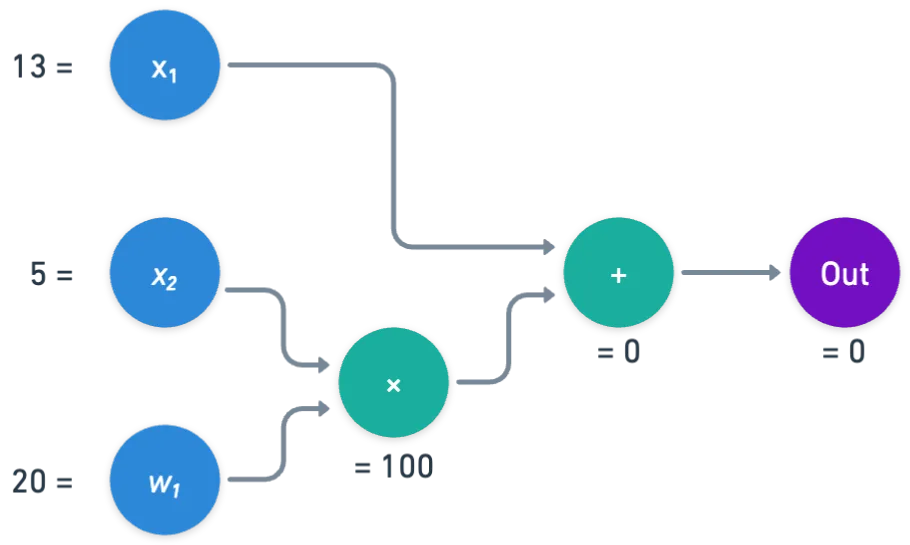
And we could think of this evaluation as the following trace, visualized as a table:
| inputs | 20 | 13 | 5 |
| left input | right input | output | |
|---|---|---|---|
| gate 0 | 5 | 20 | 100 |
| gate 1 | 13 | 100 | 0 |
The fantastic idea behind modern SNARKs, including Plonk, is to encode this trace as polynomials, which will ultimately allow a verifier to check that the computation is valid. Valid here means that a specific set of constraints are followed. Namely:
- That each gate is correctly evaluated
- That wires with the same origin have the same value
By wire, I mean the connections between gates, or connections from inputs to gates, in the circuit. We can think of these wires as holding the values of the circuit, instead of the nodes themselves:
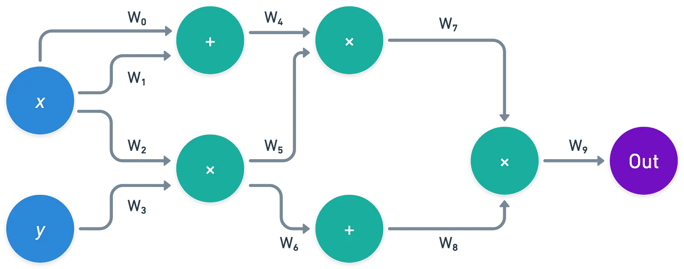
Here, you can see that some of these wires should hold the same value: , , and — and also and . Additionally, gates should make sense — meaning that, for instance, should equal .
A circuit can be either a recipe for computation, or a set of constraints to check!
Each of this sets of constraints — wire values, gate constraints, and wiring constraints — , will be encoded in different polynomials.
For example, the entire computation trace can be encoded into a single polynomial , where corresponds to one wire.
We have the wire values , but we need to choose to which values we encode them. Using some integers is a perfectly valid option — you know, the set . But there’s a lot to gain from using the roots of unity of our field instead.

Roots of Unity
I mentioned this concept before, but dodged having to explain any further like Neo in Matrix.
I think now is good time to zoom in a bit, so that we can better understand the notation coming ahead.
So, yeah, time for some definitions. We call a value (the greek letter omega) a root of unity of the field if:
In this case, the set :
doubles up as a cyclic multiplicative group, generated by :
There are two nice things about using elements of this set as the inputs to our encoding polynomial . First, moving from one root of unity to the next, is as simple as** multiplying by** . Likewise, moving backwards is done by multiplying by the inverse of . And it wraps all the way around - by definition:
Secondly — and this is the most important part — , using this set allows us to perform interpolation using the most efficient algorithm we know: the Fast Fourier Transform. We won’t dive into how it works (at least not now!), but know that this improves interpolation time dramatically — meaning that proofs are faster to generate (than other methods for interpolation).
Encoding the Circuit
Having said all this, it’s time to get down to business. Time to actually see how the computation trace is encoded.
Let’s denote the number inputs to our circuit by , and the number of gates by . With this, we define:
Each gate has three associated values: two inputs, and one output. And this is why we use . Notice that this magic number happens to be exactly the number of values in the computation trace!
We’ll encode all these values into the roots of unity:
But which root encodes to which wire? We need a plan!
- The inputs will be encoded using negative powers of . For the input , we use:
- The three wires associated to each gate , ordered as left input, right input, and output, will be encoded by the following values:
If we look at our sample trace, we’d get something like this:
With this, all the values in our computation trace are included in the polynomial. We just have to interpolate, and obtain , which will have degree .
Gate Encoding
Gates present a complication: they can be either addition or multiplication gates. This means that proving that a gate is correctly evaluated, requires us to convey information about its type.
We do this via a selector polynomial . For gate :
When the gate is an addition gate, then will take the value , and if it is a multiplication gate, then it will take the value . To make this simple to write, let’s just define:
And then construct the following expression:
Don’t let the expression scare you — what’s happening is actually fairly straightforward. You see, either or . Because of this, only one of the terms containing will be active for some gate , and in consequence, this expression ties inputs ( and ) and outputs (encoded in ) of a gate, along with the gate type.
Wiring Encoding
This one is the trickiest of the lot. As mentioned before, it may happen that some wires correspond to the same value, since they come from the same source, like this:
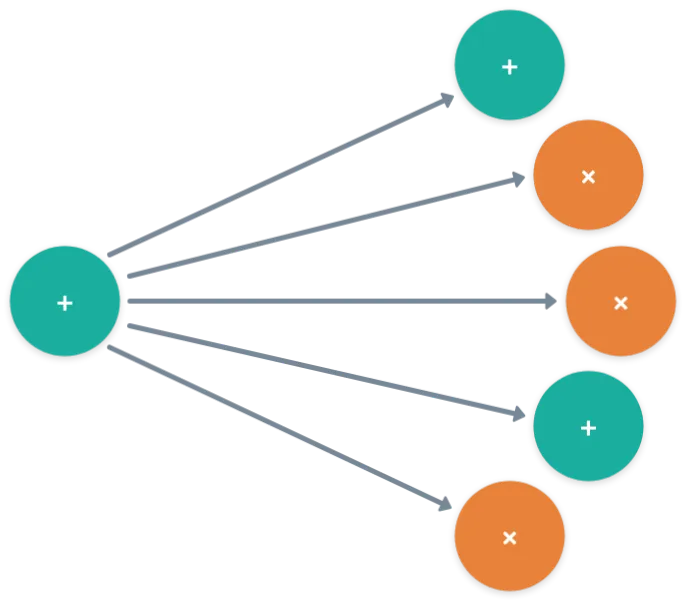
What this means is that some of the values encoded into need to match:
If we analyze the entire circuit, we’ll end up having a set of this kind of constraints:
This is for the example above. But in general, the equalities may have more than members each
Each one of these must be somehow encoded, of course, into polynomials. They way we do this is quite interesting: for each constraint, we define a polynomial that permutates or rotates the subset of roots whose evaluation should match. So for example, if the condition is:
Then we define the subset:
And using , we create a polynomial that has the following behavior:
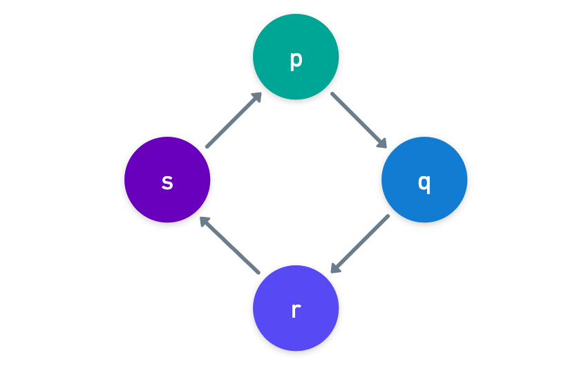
Because always returns “the next” element in , and since all the values of should be equal for the roots on , the way we prove that the wiring constraint holds is by proving that:
This has to be done for every element in , thus covering all the equalities in a single constraint.
Okay! That was certainly a lot. Nevertheless, we’ve already covered a lot of ground with this.
At this point, the prover has all these polynomials that encode the entire computation trace. What’s missing then? Only the most important part: convincing a verifier that the trace is correct. Once we understand how this happens, everything will finally be tied together.
Verification Requirements
Of course, the verifier doesn’t know the polynomials we just talked about. In particular, it’s critical that they never learn the full . The reason for this is that, if they do get ahold of it, then they could easily uncover the secret information , by calculating:
The ability to never reveal these values by using polynomials is what gives Plonk its zero knowledge properties!
If the verifier cannot know the polynomials, then how can we convince them of anything? Did we hit a dead end? Should we panic now?

While the verifier cannot ask for the full polynomials, they for sure can ask for single evaluations of them. They should be able to ask for any value of , , or the 's — meaning they should be able to query any part of the computation trace. Except for the secret inputs, of course.
It’s at this point that our PCSs of choice comes in handy: when requesting the value of at some point (so, ), the verifier can check that it’s correctly computed by checking it against a commitment! Noooice.
Why would they do that, though? To check that the constraints hold, that is!
To be convinced that the computation trace is correct, the verifier needs to check that:
- The output of the last gate is exactly (this is a convention),
- The inputs (the public ones, or the witness) are correctly encoded,
- The evaluation of each gate is correct (either addition or multiplication holds),
- The wiring is correct.
The first one is easy — the verifier just asks for the output at the last gate, which is:
For the other checks though, we’ll need to sprinkle in some magic (as usual, at this point).

The Last Sprinkles of Cryptomagic
We’ll need to sidetrack a little for a moment. Here’s a question: given some polynomial of degree at most , and that is not identically (so ), how likely would it be that for a random input (sampled from the integers modulo ), we obtain that ?
Because the polynomial has degree at most , it will have at most roots. Then, the probability that is exactly the probability that happens to be a root of :
And provided that is sufficiently larger than , then this is a negligible value (very close to zero). This is important: if we randomly choose some and obtain that , then we can say with high probability that is identically zero (the zero function)!
This is known as a zero test. It doesn’t seem to amount to much, but we’re gonna need this to make our SNARK work.
There are a couple more checks that we can perform, namely an addition check, and a product check. This is already quite a lot of information to digest, so let’s skip those for now.
What interesting is that there are efficient Interactive Oracle Proofs to perform these tests.
Sorry... Interactive WHAT?

Interactive Oracle Proofs
I warned you this wasn’t gonna be easy! Just a little bit more, and we’re done.
Interactive Oracle Proofs (IOPs) are essentially a family of mechanisms, by which a prover and a verifier interact with each other, so that the prover can convince the verifier about the truth of a certain statement. Something like this:
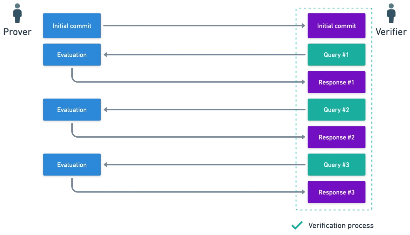
I hope you can already see how this picture looks similar to the one we used to describe Polynomial Commitment Schemes (PCSs)!
And we’ll use this model to perform our tests. For illustrative purposes, let’s describe how a zero test would go.
Imagine you want to prove that some set is a collection of roots of a given polynomial :
What can you do about it? Well, since the values in are roots, you can divide the polynomial by what’s called a vanishing polynomial for the set :
The term vanishing is due to the fact that the polynomial is zero only on the set , so they are exactly its roots.
If really are the roots of , then should be divisible by , with no remainder.
And now, we’re gonna have to use a Polynomial Commitment Scheme to continue. You might have to read that article first!
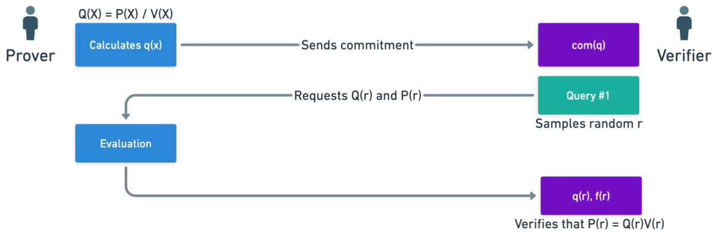
Essentially, what happens is that the prover commits to both and , and then, they request an evaluation at some random . With these evaluations, they can check whether if the following is true:
If it happens to be zero, then we saw that they can conclude with high probability that this polynomial $Q(X)V(X) - P(X)* is exactly zero! Meaning that:
Thus, they can be convinced that, effectively, is a set of roots of . If for some reason they aren’t convinced though, they could ask for another set of evaluations of and , and run the check again.
Similar IOPs exist for the addition check and the product check.
Also worth mentioning, this does not ensure that the polynomial doesn’t have other roots that are not contained in . But we’ll not go down that path this time around!
From Interactive to Non-interactive
But wait... Didn’t we say that SNARKs were non-interactive? Then how is it possible that some interactive protocol is a key part of our construction?
Turns out there’s a way to turn interactivity into non-interactivity: the Fiat-Shamir transform. It sounds more daunting than what it is, trust me.
If we think about it, we may wonder “why are these protocols interactive in the first place?” The reason is that on each query, the verifier samples some random number from some set. And these values cannot be predicted by the prover — they only become available for them when the verifier chooses to execute a query. This unpredictability is sort of an anti-cheat mechanism.
Instead of waiting for the verifier to send random values, we can simulate this randomness using a well-known cryptographic primitive that also has an unpredictable output: hashing functions!
Let’s not focus on the details though — all you need to know is that the Fiat-Shamir heuristic is a powerful transformation, that can be very useful to turn any interactive protocol into a non-interactive one!
After what can only be categorized as torture, we have all the elements we need. Our excruciating journey is almost over — all that remains is putting the cherry on top of this pile of shenanigans.

Back to Verification
Okay, let’s see. Remember, we’re trying to convince a verifier that we know such that:
And we have to convince them of a few things:
- Correct inputs
- Correct gate computation
- Correct wiring
Let’s start with the inputs. The verifier has the public witness, . Now, imagine the verifier encodes this witness into a polynomial , so that:
In this scenario, it should be true that values and match for the roots of unity that encode the public witness:
So what do we do? Why, of course, a zero test for the polynomial on the inputs that encode the witness!

Ahá! It’s starting to come together, isn’t it?
Checking the Gates
Likewise, recall that the gates should suffice the expression:
So again, what do you do? A zero test on this massive expression, on every gate. Marvelous. Splendid.
For this of course, the verifier will need a commitment to .
Checking the Wires
Lastly, we need to check the wire constraints. These were encoded into some polynomials that cycled through a set of inputs , and we had to check that:
For each element in . This is not really efficient to do with zero tests (although it can be done), so there’s an alternative way to do it through the use of a product check. Using this casually dropped expression:
Yeah
The gist of this is that the whole expression should equal ! If you think about it, it makes perfect sense: all the values should be the same, and since permutates the elements of , and because the product covers all of , we just get:
There’s more to say about this, like why do we need to incorporate and into the mix? But honestly, I think that’s enough math for today.
In short, and to wrap things up: we use some IOPs to verify the constraints in an arithmetic circuit, which were encoded into polynomials!
Summary
Ooof. That was a lot. I know.

Still, I find it amazing how all these things come together to form such a sophisticated protocol: we use polynomial interpolation to encode stuff, polynomial commitment schemes to query for information, interactive oracle proofs to create tests, and the Fiat-Shamir heuristic to turn all this mess into a non-interactive proof. Un-be-lie-va-ble.
The final result, Plonk, achieves the generality we were looking for by allowing any circuit to be used. And since this reveals nothing about , then this is really a zero-knowledge SNARK (zkSNARK)!
For the sake of completeness, I’ll say that there are some other details to be considered in order to make sure that the protocol is zero-knowledge, specifically around the challenges. Don’t worry too much though — unless, of course, you’re planning on implement Plonk yourself!
For a more interactive look, you can check this excellent video lesson.
And here’s another stab at explaining the protocol, in case you find it easier to follow!
Hopefully, you can now better understand the brief description of Plonk I provided at the very beginning of the article:
![]()
![]() In Plonk, we encode the computation of a circuit into a series of polynomials, which represent the constraints imposed by the circuit, for which we can prove statements by using a series of tests, without ever revealing the polynomials themselves— and thus, not leaking the secret inputs.
In Plonk, we encode the computation of a circuit into a series of polynomials, which represent the constraints imposed by the circuit, for which we can prove statements by using a series of tests, without ever revealing the polynomials themselves— and thus, not leaking the secret inputs.![]()
![]()
Given that we can now craft proofs for arbitrary circuits, I’d like to get more practical. So, next time, we’ll be building a couple circuits for some statements, which can then be the inputs for Plonk, turning them into zkSNARKS. See you soon!


Did you find this content useful?
Support Frank Mangone by sending a coffee. All proceeds go directly to the author.