The ZK Chronicles: Multilinear Extensions

---

In the previous installment, we saw our first instance of a protocol that makes use of a general model for computation: circuits.

Although interesting in concept, we noted that ideally we’d like to prove that a computation, represented as a circuit, was correctly executed — not that we know how many inputs satisfy the circuit (recall we studied #SAT).

The question though, is whether we can do that with our current knowledge. And well... We can’t!

It feels we’re really close though, and to be fair, we are. However, getting there will require using a little mathematical gadget we haven’t talked about so far.

Even though things might be a little heavier on the math side today, don’t lose sight of our endgame: to prove we have a satisfying input for some circuit!

And so, it’s time for us to make a new acquaintance: a little tool that will be very helpful in our upcoming efforts.

Into the action we go!

Building Intuition

During the sum-check article, I mentioned how $0$ and $1$ were two special inputs because of how easy it was to evaluate polynomials at those points.

But let’s be honest: in most real-world scenarios, we don’t actually care about evaluations at $0$ and $1$ specifically. They’re just numbers like any other — they don’t have any inherent semantic meaning.

The same does not really apply to boolean circuit satisfiability, since the inputs are truly boolean variables to begin with!

So when sum-check asks us to verify sums over a boolean hypercube, an obvious question arises: who even cares?

When would we ever need to sum a polynomial over these specific points?

The answer might surprise you: all the time freakin’ time. But to make sense out of all this, we need to look at those boolean hypercubes in a different light.

Encoding Information

The key to this matter is to view them as a way to encode information.

Let’s look at a concrete example: a simple list of numbers. Suppose we have a small list of four values, say $[2, 3, 5, 8]$. To access a specific value of that list, you’d normally provide an index. So for example, to retrieve the value $5$, you’d request the value in the list at index $2$.

Assuming we’re using zero-indexing, of course!

Now, here’s an observation: the indexes are just integers, and these all have binary representations. What’s more, this little list has 4 possible indexes, which would look like this in binary:

• Index $0$ → $00$
• Index $1$ → $01$
• Index $2$ → $10$
• Index $3$ → $11$

You see where I’m going with this, right? Each index is just a point in the boolean hypercube $\{0,1\}^2$ !

Same information, different representation!

With this, we can imagine the action of reading the information in our list at a given index as a function, where we can already assume the indexes are values in the hypercube (which in this case, is just a boolean square):

$$f: \{0,1\}^2 \rightarrow \mathbb{F}$$

Which is just math notation for saying “a function $f$ that takes two boolean variables, and returns some value in a field”.

So, following the example, we have:

• $f(0,0) = 2$
• $f(0,1) = 3$
• $f(1,0) = 5$
• $f(1,1) = 8$

Okay, okay. But isn’t this just more pointless relabeling?

Actually, no! You see, the real kicker here lies in that little function $f$ we’ve so inconspicuously slid into view. Implicitly, we’re saying that this function is able to encode data.

In fact, we’ve seen a method to obtain said function: interpolation. Obviously, what we obtain from that process is a polynomial. And it is through this type of encoding that the sum-check protocol will become relevant.

Cool! Slowly but surely, it seems we’re getting somewhere.

But I want you to notice something: back in our pass through Lagrange interpolation, we actually focused on the univariate case. Interpolation was presented as a way to obtain a univariate polynomial from evaluations, which we treated as $(x, y)$ pairs.

In the sum-check protocol though, we make use of some polynomial $g$ with $v$ variables, rather than a single variable. So here, interpolation as we described it will not get us to the type of polynomial we need.

Thus, we’re gonna need something different.

Multilinear Extensions

What we need is a way to go from a multivariate function (like our $f$ above) defined over a boolean hypercube to a multivariate polynomial. We’ll call said polynomial $g$ for convenience, given our parallel with sum check.

And we’ll do this in a very special way. Because there are two important conditions to consider here:

• Agreement on the hypercube: we want to encode some data, meaning that $g$ must match a set of values at the boolean hypercube.
• Extension beyond the hypercube: in the sum-check protocol, we are required to evaluate $g$ at points other than boolean strings.

Combined, these two conditions precisely define the behavior of $g$:

It needs to be a multivariate polynomial where each input can be a finite field element, and whose outputs match the encoded values at the boolean hypercube

Yeah... That’s a mouthful. Let’s unpack.

First, we’re saying that we need some function defined over these sets:

$$g: \mathbb{F}^v \rightarrow \mathbb{F}$$

This is, it takes v inputs in the field $mathbb{F}$, and will allow us to encode a total of $2^v$ values. And for those values, we have a series of restrictions to the function:

• $g(0, 0, ..., 0, 0)$ encodes $f(0, 0, ..., 0, 0) = k_0$, so $g(0, 0, ..., 0, 0) = k_0$, where $k_0$ is some element in $mathbb{F}$.
• Then, $g(0, 0, ..., 0, 1)$ encodes $f(0, 0, ..., 0, 1) = k_1$, so $g(0, 0, ..., 0, 1) = k_1$.
• Likewise, $g(0, 0, ..., 1, 0) = k_2$.
• $g(0, 0, ..., 1, 1) = k_3$

And so on. Thus, we require that:

$$f(w) = g(w) \ \forall w \in \{0,1\}^v$$

Which is just math notation for: $g = f$ only on the hypercube.

This is the construction we’re after. It’s as if we’re extending our original function $f$ so that the inputs can take values other than $0s$ and $1s$, allowing values on the larger finite field. Hence the name: multilinear extensions.

But wait, why multilinear? What does that even mean?

Multilinearity

Before any confusion happens: multivariate and multilinear are not the same thing.

Polynomials can have, as we already know, different degrees, as the different terms in the expression itself can be raised to different integer powers. We could even stretch language a bit here and talk about the degree of each variable, as the maximum power a given variable is raised to throughout the whole thing.

Saying that a polynomial is multilinear actually poses a strong restriction on how the expression can look: what we’re saying is that the degree of each variable is at most $1$. To be perfectly clear, this is a multilinear polynomial:

$$g(X_1, X_2, X_3, X_4) = X_1X_4 + X_2X_4 + X_3X_4$$

And this is not:

$$g’(X_1, X_2, X_3, X_4) = X_1²X_4 + X_2X_4 + X_3X_4$$

That single term with $X_1^2$ makes the entire polynomial non-linear!

Alright... But, again, why does this matter?

Turns out that imposing this condition has a couple nice consequences. You see, in principle, we could extend our original function $f$ using polynomials of any degree. In fact, there are infinitely many ways to do this!

Take for example our 4-element list $[2, 3, 5, 8]$. We could build polynomials such as:

• $g_1(X_1, X_2) = 2 + X_1 + 3X_2 + X_1X_2$
• $g_2(X_1, X_2) = 2 + X_1^3 + 3X_2 + X_1X_2^5$
• $g_3(X_1, X_2) = 2 + 100X_1^7 + 3X_2 {-} 99X_1^7 + X_1X_2$

All three correctly encode the list on $\{0,1\}^2$, and of course diverge everywhere else. So... What’s makes multilinearity special, specifically?

First of all, there’s the fact that a multilinear expression is simple and efficient. These polynomials will require evaluation at some point, and in that regard, degree matters. Multilinear polynomials tend to be less expensive to evaluate than higher-degree expressions, plus they generally have less coefficients, which also impacts communication costs.

Plus, some soundness arguments rely on some polynomials having low degree!

But this isn’t all. When we restrict ourselves to multilinear polynomials, it just so happens there is only one way to define $g$ so that it matches all our requirements. In other words, a multilinear extension (or MLE for short) of some function $f$ defined over the boolean hypercube is unique.

Heck, let me put it in even stronger terms:

There’s a natural, unique way to extend a function $f$ defined on a boolean hypercube to a multilinear polynomial

This is powerful. So much so, that I think we should prove this statement.

Feel free to skip this next section. I just think it’s worthwhile, since it’s such a useful property of multilinear extensions!

Uniqueness

To show this, we’ll first need a strategy to build such a function $g$.

Here’s what we’ll do: for each point $w$ in $\{0,1\}^v$, we’ll build a polynomial that evaluates to $1$ on $w$, and to $0$ everywhere else on the hypercube.

That must sound familiar. Can you remember where we saw something similar?

Yes, that’s exactly how we defined Lagrange bases! That’s pretty much what we’re doing here.

Alright then, let’s define that:

$$\chi_w(X_1, ..., X_v) = \prod_{i=1}^{v} [w_iX_i + (1-w_i)(1-X_i)]$$

That might look a little odd, but it works just fine:

• When the $X$ values are the coordinates of $w$, each term evaluates to $w_i^2 + (1 {-} w_i)^2$. Note that this equals $1$ when $w_i$ is either $0$ or $1$. Thus, the entire product results in $1$.
• When $X$ takes some other value different than $w$, then at least one $X_i$ is different from $w_i$, so either $X_i = 0$ and $w_i = 1$, or vice versa. In both cases, $w_iX_i + (1 {-} w_i)(1 {-} X_i)$ equals $0$, thus collapsing the entire product to $0$.

To get our extension, we just need to add all these terms together, multiplied by the encoded value at a given index, $f(w)$:

$$g(X_1, ..., X_v) = \sum_{w \in \{0,1\}^v} f(w) \chi_w(X_1,...,X_v)$$

You can check for yourself that this expression is multilinear. And as such, we have constructed a valid MLE of $f$!

What remains is proving that this expression is the only possible MLE for $f$.

I’ll start abusing notation a bit now, to keep things a bit more condensed. When I say $p(X)$, just assume $X$ is a vector. This makes sense in the context we’re working with, after all!

To do this, we’ll do something quite clever. Suppose $p(X)$ and $q(X)$ are two valid MLEs for $f$. From them, let’s build this polynomial $h$, which is also multilinear:

$$h(X) = p(X) {-} q(X)$$

Because $p(X)$ and $q(X)$ are valid MLEs, they have the same values on the boolean hypercube, meaning that those values will be roots of $h(X)$.

Most commonly, this is stated as: $h(X)$ vanishes at $\{0,1\}^v$.

To prove $p(X)$ and $q(X)$ are the same polynomial though, we need to show that $h(X)$ is identically $0$ — that is, its expression is $h(X) = 0$.

Now, since $h(X)$ is multilinear, it has degree at most $1$ in each variable — so its total degree is at most $v$. As we already know, a non-zero polynomial of degree $v$ can have at most $v$ roots.

But... We’re claiming $h(X)$ has $2^v$ distinct roots!

That’s impossible: $2^v$ is greater than $v$ (for any $v \geq 1$). Unless, of course, we allow $h(X)$ to be the zero polynomial!

Therefore, the only possibility here is that $h(X) = 0$, which in turn means that $p(X) = q(X)$. Thus, the MLE is unique, and is exactly the expression we built.

Neat, eh?

Uniqueness is important because it prevents forgery. By this, I mean that if multiple possible extensions existed, a cheating prover could try to build one to suit their devious needs.

But with MLEs, there’s only one correct extension. The extension process gets protection for free: uniqueness means no wiggle room for cheaters!

Computing MLEs

Alright! We’ve shown that MLEs are unique and well-defined. But there’s something else we need to address: practicality.

Let’s take another quick look at our formula:

$$g(X_1, ... \ , X_v) = \sum_{w \in \{0,1\}^v} f(w) \chi_w(X_1, ... \ ,X_v)$$

Note that we’re summing over $2^v$ elements, and each of the $\chi$ terms involves $v$ multiplications. Naively, evaluating a single point in $g$ would take a total of $O(v.2^v)$ operations. If we’re not careful about how we use these extensions, computational costs could explode, rendering MLEs impractical.

Fortunately, there’s a clever optimization to compute MLEs that brings down evaluation times dramatically, and this is what ultimately makes these little guys very useful.

The trick, once again, has to do with a recursive structure we can exploit. An example here will help conceptualize the general idea.

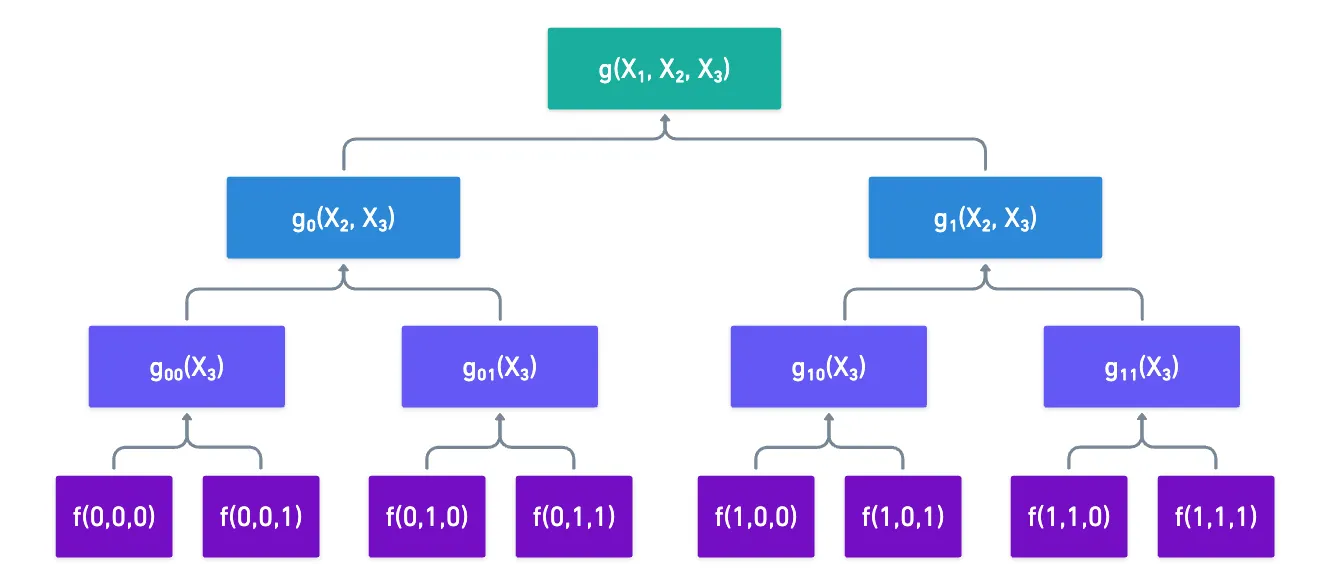
Suppose we want to compute the extension $g(X_1, X_2, X_3)$ of some 3-variable function $f$. The fact that each variable is binary allows us to write $g$ in this way:

$$g(X_1, X_2, X_3) = (1 {-} X_1)g_0(X_2, X_3) + X_1g_1(X_2, X_3)$$

Where $g_0$ and $g_1$ are restrictions of the original function $g$ at $X_1 = 0$ and $X_1 = 1$ respectively.

By using these restrictions, we’ve split the evaluation of our original MLE into the evaluation of two smaller MLEs! Of course, we don’t need to stop there: we can now take $g_0$ and $g_1$, and do the exact same thing, reducing their evaluation to two new MLEs with one less variable.

$$g_0(X_2, X_3) = (1 {-} X_2)g_{00}(X_3) + X_2g_{01}(X_3)$$

Once we get to univariate polynomials, their evaluation becomes super simple:

$$g_{01}(X_3) = (1 {-} X_3)f(0,1,0) + X_3f(0,1,1)$$

Remember: $X_3$, as well as the other variables, will take values from the finite field when we’re computing the multilinear extension — not only $0$ and $1$!

So, in order to evaluate $g$, we have to go in the opposite direction. We start with the evaluations of $f$, and we take combinations of them. Following through our example would result in this little graph here:

Click to zoom

The magic happens when we consider the context in which these MLEs are used. You see, in our good ol’ sum-check protocol, we need to calculate $g$ at points like these in subsequent rounds:

• $g(0, 0, 0), g(0, 1, 0), g(0, 0, 1), g(0, 1, 1), g(1, 0, 0), ...$
• $g(r_1, 0, 0), g(r_1, 1, 0), g(r_1, 0, 1), g(r_1, 1, 1)$
• $g(r_1, r_2, 0), g(r_1, r_2, 1)$

If you need to, go check the protocol again!

On each round, one variable is fixed to a challenge value $r$, but the remaining variables still take boolean combinations that are repeated, and can be reused.

We can see this in action in our little example. Suppose we need to find $g(0,0,0)$, and then $g(r_1,0,0)$. The first evaluation prompts us to calculate $g_0(0,0)$ and $g_1(0,0)$:

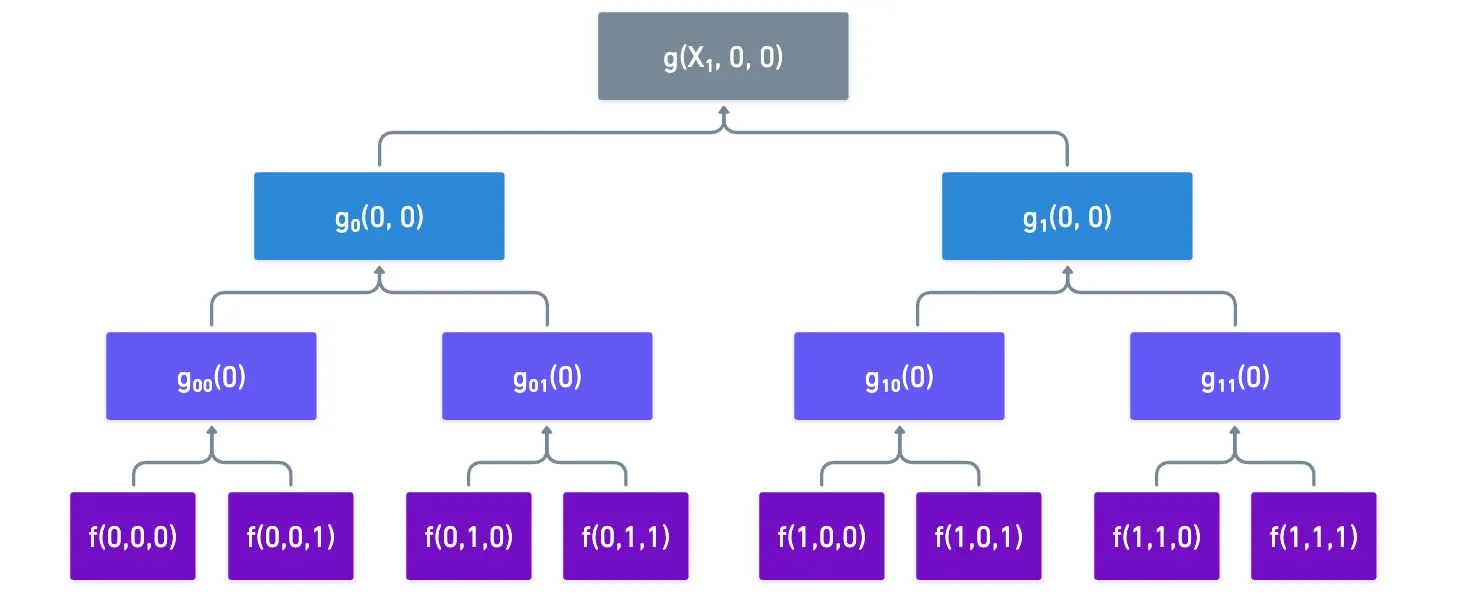
If we store those values for later use, we can simply reuse them when we’re required to calculate $g(r_1,0,0)$:

$$g(r_1) = (1 -r_1)g_0(0,0) + r_1g_1(0,0)$$

What we’ve done is use one of the oldest tricks in the book in algorithm design: memoization!

All we do is store intermediate values when we execute the full evaluations at the beginning of the sum-check, and then we simply reuse them later, significantly cutting down evaluation costs!

This gained efficiency mainly helps keep the prover’s runtime manageable during the sum-check protocol, or really, in any other context where we encode data in this binary fashion.

Cool! We’ve now covered most of the tricks behind MLEs. But before we go, we’ll need to talk about just one more little thing, which happens to be a fundamental we’ll use a lot moving forward.

The Schwartz Zippel Lemma

The insight we used moments ago to prove uniqueness — that a non-zero polynomial of degree $d$ can have at most $d$ roots — is actually a special case of a more general and powerful result we’ll use many times throughout the series, called the Schwartz-Zippel lemma. And now’s the perfect time to present it!

Here’s the idea: if $p(X_1, ..., X_v)$ is a non-zero polynomial of total degree $d$ over a field $\mathbb{F}$, and we pick random values $r_1$, $r_2$, ..., $r_v$ from $\mathbb{F}$, what’s the probability that we happen to land on a root?

This value happens to be exactly:

$$\textrm{Pr}[p(r_1, ..., r_v) = 0] \leq d / |\mathbb{F}|$$

As long as $d$ is much smaller than the size of the finite field, then this probability is negligible! Thus, if we choose a random set of inputs, and we actually get $p(r_1, ..., r_v) = 0$, then there’s a really high chance that the original polynomial was the constant polynomial $p(X_1, ..., X_v) = 0$!

This seems simple, but it’s actually a super powerful tool. One very simple application is showing that two polynomials are identical: given $p(X)$ and $q(X)$, we can define $h(X)$ as:

$$h(X) = p(X) {-} q(X)$$

When we select a random point $r*$, and check that $p(r*) = q(r*)$, we’re in fact saying that $h(r*) = 0$, which means with high probability that $p(X)$ equals $q(X)$.

This should be very reminiscent of the reasoning we used during the soundness analysis of the sum-check protocol. Although we didn’t say it explicitly, we used the Schwartz-Zippel lemma!

We’ll use this a lot, so definitely keep this one in mind!

Summary

Alright, that was probably a lot! Let’s take stock of what we’ve learned today.

First, the boolean hypercube works well as an indexing strategy. We could leverage that to encode information, since the index could serve as an input of some function, and the data we wanted to encode could be its output.

Then, to use this function in sum-checking, we identified it needed to be extended. This is how we arrived at multilinear extensions: unique extensions of these functions no longer bounded to a boolean hypercube.

Though I didn’t mention it explicitly, it’s very easy to construct these MLEs. The Lagrange bases we used are super simple. For this reason, MLEs are the superior choice when extending functions!

With MLEs, we can take just about any dataset — a database, a vector, a matrix — and encode it as a polynomial that can somehow work well with sum-checks.

Obviously, there’s something we haven’t addressed yet: what role do sum checks play in all this?

I mean, encoding data is fine and everything, but where’s the computation?

That’s where circuits come in. And that will be our next stop, where things will finally start clicking into place!

See you on the next one!