The ZK Chronicles: Sum Check

---

Now that we’re equipped with finite fields and polynomials, it’s time to take a look at our very first proving system. Yay!

Truth is, the tool we’re about to present might feel a bit pointless at first glance. When studied in isolation, it will feel like an extremely convoluted way to perform a very simple task.

Don’t let that discourage you though! As it happens, this tool is extremely important for a wonderful reason: many problems we want to prove things about can be reduced to a version of what we’re about to unveil.

Therefore, I ask you to approach today’s article with an open mind. Think of today’s topic as just another stepping stone in our path to obtaining useful proving systems.

Things will start clicking in very soon, I promise. Trust the process!

Alright then! Expectations are high, so let’s waste no time. Let’s talk about the sum-check protocol.

Getting Started

As a short reminder of our very first encounter, what we want to do is build some sort of proving system to show that the result of some computation is valid, and do so in less time than the computation itself, ideally.

Cool, so... What kind of computation are we talking about?

So far, our toolkit only includes polynomials. Using these as a basis, we could try to come up with ways of representing useful computations — the kind we can prove things about.

Okay then, let’s start small. Take some univariate polynomial $P(X)$. Perhaps the simplest thing we can do with it is to evaluate it at some point. And on that account, I want to note that there are two special points with an interesting behavior upon evaluation: $0$ and $1$.

Think about it for a second: when $X = 0$, all terms containing $X$ just vanish, leaving us with the term with no $X$. This is usually called the constant term, or the zeroth coefficient.

Likewise, evaluating a polynomial at $X = 1$ simply gives us the sum of all the coefficients in the polynomial!

Essentially, these points are nice because we don’t need to spend time calculating any powers of X during evaluation. Granted — we could use any other point, but these just happen to be convenient, and very important for today’s construction.

I know. Not the most fun stuff, but it’s a start.

The next thing we might try is adding evaluations together. For instance, we could have:

$$P(0) + P(1) = k$$

Where $k$ is some field element. Performing this calculation directly is quite easy for the reasons we stated before: evaluation is very straightforward. It seems we’re not really making much progress — after all, we said that proving a result makes sense only when there’s a real gain in verification time versus computation effort.

And here, computation is so simple that it’s kind of absurd to try and build a separate algorithm for verification.

I mean, just look at the expression above!

So how about we kick it up a notch?

Turning Up the Heat

What would happen if our starting point was a multivariate polynomial instead? Something like this:

$$g(X_1, X_2, X_3,...,X_v)$$

Now we’re talking.

In terms of evaluation complexity, we’re pretty much in the same situation as before: it’s quite simple to evaluate these polynomials at variable values $0$ and $1$.

But the situation changes when we consider combinatorics. Since we now have $v$ variables, and each can be either $0$ or $1$, we now have $2^v$ possible combinations to evaluate!

These points, represented as the set $\{0,1\}^v$, form what’s called the boolean hypercube.

Calculating this sum does indeed take some more work:

$$H = \sum_{b_1 \in \{0,1\}} \sum_{b_2 \in \{0,1\}}...\sum_{b_v \in \{0,1\}} g(b_1, b_2, ..., b_v)$$

In Big O terms, we can say that calculating $H$ takes exponential time $O(2^v)$. Meaning it takes at least $2^v$ evaluations.

I’ll assume familiarity with this notation, but as a short explainer, what it does is express complexity based on the term in an expression that grows the fastest.

As variable values increase, said term will grow bigger (more significant) than others, rendering every other term negligible in comparison.

So for example, take $2X^2 + X$. As $X$ grows larger, $X^2$ grows much more rapidly than $X$ — and soon enough, $X^2$ will be much bigger than $X$. Thus, we say the complexity of the expression is $O(X^2)$. Notice we ignore multiplicative factors, as they don’t affect the behavior of the function — they only scale it.

For very large values of $v$, exponential time can be a really long time.

Prohibitively long for my poor computer, but maybe not for someone with some heavy-duty hardware.

In this context, it does make sense to try and fabricate an algorithm for fast verification of some claimed result.

And this is exactly the goal of the sum-check protocol!

Let’s see how it works.

The Protocol

A protocol is simply a sequence of steps, defined by rules that must be followed during an interaction between parties. This is exactly our situation: a prover and a verifier will interact in a very specific manner.

The beauty of this protocol we’re about to present lies in its recursive nature.

Here’s the plan: we’ll first explain how a single round works. Once we finish with that, it will be immediately clear that to continue moving forward, we’ll have to do another one of those rounds. Each round will sort of reduce the problem, until we’re left with a condition that’s very simple to check.

Click to zoom

Easy, right?

Woah, woah, chill... Okay, one step at a time.

A Sum-Check Round

The setup is the following: a prover claims to have calculated the sum $C$ for a polynomial $g(X_1, X_2,..., X_v)$ over $\{0,1\}^v$. Their goal is to convince a verifier that $C$ is the correct result.

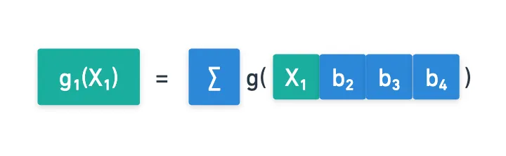
To do so, the prover will do something quite strange in appearance: a partial sum of $g$.

$$g_1(X_1) = \sum_{(x_2, ..., x_v) \in \{0,1\}^{v-1}} g(X_1, x_2, ..., x_v)$$

If you look closely, you’ll notice that we have not included evaluations for the first variable, X_1. For this reason the result is a new polynomial — a univariate one, specifically.

Click to zoom

Believe it or not, this is all they have to do. The prover can send $C$ and $g_1(X_1)$ to the verifier, and with these values, the verifier can easily check the following equality:

$$C = g_1(0) + g_1(1)$$

Clearly, if $C$ is correctly calculated, this equality should hold (feel free to check that yourself if you’re not convinced!). So if this test passes, we’re done! The verifier can confidently say that $C$ is correct!

Or... Can they?

Problems in Paradise

In fact, there’s a critical issue with this reasoning — and it’s a consideration we need to always keep in mind as we move forward in our journey. We’ve said it before, but I’ll say it again, and in big letters, so you guys don’t ever forget:

The prover could be lying

What could they be lying about? Well, just about everything they can lie about — but in this case, they don’t have many options: they either don’t know $g$, or they lie about the value of $C$.

So, let’s say the prover wants to convince the verifier that some value $C^*$ is the correct result, but is in fact incorrect. How would they go about it?

Pretty much the only knob they can control is that polynomial $g_1(X_1)$. And if you think about it, nothing stops the prover from crafting a simple polynomial $g_1^*$ so that the verifier check passes!

$$C^* = g_1^*(0) + g_1^*(1)$$

It wouldn’t even be that hard!

As things are right now, the algorithm won’t work. We’re gonna need a way to check that $g_1(X_1)$ was correctly calculated.

Let’s take a moment to ponder our options. Naturally, verifiers can’t trust a prover’s word. And $g_1(X_1)$ is just a polynomial — all we can do with it is evaluate it at some point.

Wait... What happens if we evaluate $g_1(X_1)$ at some random point $r_1$?

$$g_1(r_1) = \sum_{(x_2, ..., x_v) \in \{0,1\}^{v-1}} g(r_1, x_2, ..., x_v) = C_2$$

Do you see it? A little miracle has unfolded before our eyes: we’re back where we started!

Yeah, sorry. Let me explain.

Once we choose and fix a random point $r_1$, the evaluation $g_1(r_1)$ is actually a sum over a reduced boolean hypercube. It's as if we're replacing the original function $g$ for another function $g'$ with one less variable:

$$g’(X_2, ..., X_v) = g(r_1, X_2, ..., X_v)$$

Now, we can ask the same original question: can we prove this reduced version of $g$ sums up to $C_2$ over a reduced boolean hypercube?

And the magic, my friends, is that another round of sum-checking does the trick!

The Full Picture

What I’m getting at here is that we can do this over and over in a recursive manner, reducing the number of variables in $g$ by one on every round. Therefore, after $v$ rounds, we’ll be left with a single evaluation of $g$.

Before tying things up, I believe seeing this in action with a simple example will help a lot.

Take for instance this polynomial of degree $4$:

$$g(X_1, X_2, X_3, X_4) = X_1X_4 + X_2X_4 + X_3X_4$$

This polynomial has to be defined over some finite field, so let’s choose a simple one, like $\mathbb{F}_{13}$.

First, the prover needs to compute the sum over the boolean hypercube ${0,1}^4$.

That’s a total of $16$ evaluations added together!

Feel free to do the calculation yourself — but in the spirit of seeing the proving system in action, let’s say the prover claims the result to be $C_1 = 12$.

The prover also sends the polynomial $g_1(X_1)$, and claims it to be $4X_1 + 4$. The verifier then simply checks:

$$g_1(0) + g_1(1) = 4 + 8 = 12$$

Okay, first round, done. Now the verifier picks a random value $r_1$. Let’s suppose that value is $r_1 = 5$.

The prover then calculates $C_2$, which happens to yield $C_2 = 11$. So now, the prover has to calculate this polynomial here:

$$g_2(X_2) = \sum_{(x_3, x_4) \in \{0,1\}^2} g(r_1, X_2, x_3, x_4)$$

The result of this is $g_2(X_2) = 2X_2 + 11$.

And we can easily calculate this because we, as provers, know the original $g$.

If we didn’t know $g$, then this random selection of $r_1$ would already make life hard for us! This type of “challenge” interaction is very important, and we’ll formalize it later.

Cool! We now check whether:

$$g_2(0) + g_2(1) = 11$$

Although the result seems to be wrong (we get $24$), everything clicks once we remember we're working on a finite field, so $24 \ \textrm{mod} \ 13 = 11$.

For the third and fourth rounds, we just rinse and repeat. To keep things brief, I'll just summarize the steps:

• Verifier chooses $r_2 = 3$.
• Prover responds with $C_3 = 4$, and $g_3(X_3) = X_3 + 8$.
• Verifier checks $g_3(0) + g_3(1) = 4$, and chooses $r_3 = 7$.
• Prover responds with $C_4 = 2$ and $g_4(X_4) = 2X_4$.
• Verifier checks $g_4(0) + g_4(1) = 2$, and chooses $r_4 = 2$.

The full process looks like this:

Click to zoom

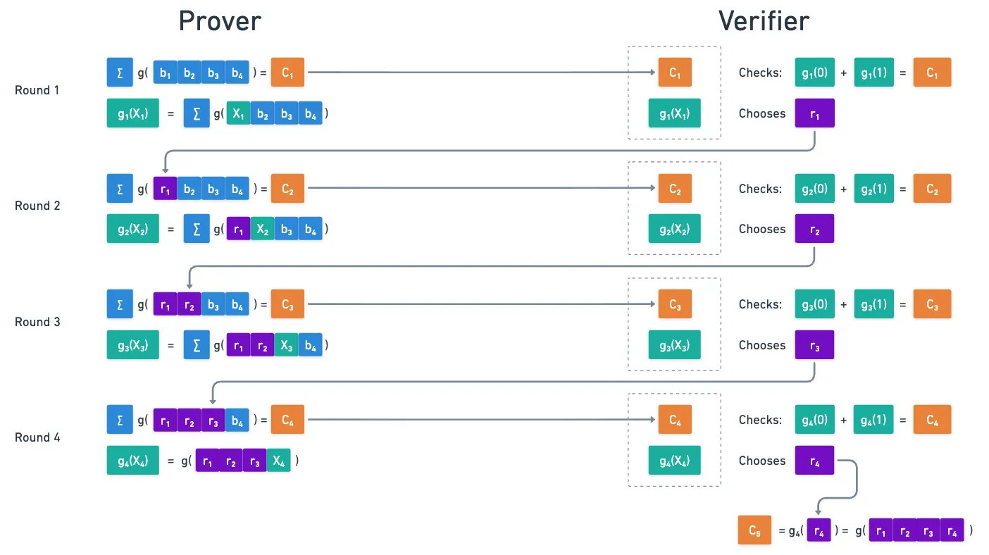
Everything checks out nicely so far. But we have a little problem: we’ve run out of variables!

Closing the Loop

Right — the original polynomial cannot be reduced any further. The verifier has received $g_4(X_4) = 2X_4$, and they need to check whether $g_4(2)$ (which in this case, equals $C_5 = 4$) is truly the same result as evaluating $g(5,3,7,2)$.

Since we cannot perform another round, it looks like we don’t have any options to check the validity of this last value. And this is not cool: what if the value is just made up so that everything works?

At this point, we’re gonna need a different strategy.

We need a mechanism to verify that $C_5$ is correct. Note that $C_5 = g(5,3,7,2)$. If there was some magical way to safely evaluate $g$ at that input, then we could compare with $g_4(2)$, and nicely close the procedure.

Sadly though... It’s too early in our journey to see how this can be achieved mathematically.

Rather than asking you to run on trust me bro vibes though, I propose the following: let’s put a name on this, so that we don’t forget about it. And when the time comes, we can circle back to this concept, and truly tie everything together.

We’ll say that we have oracle access to $g$. By this, we mean that we have a way to evaluate $g$ at some random point, and we’re guaranteed to have a correct value.

So finally, after all the checks in every round, the verifier performs an oracle query of $g$ at $(r_1, r_2, r_3, r_4)$, and accepts the proof if the value matches $C_5 = g_4(r_4)$.

Of course, this whole procedure can be generalized to any degree — and the time savings become more relevant the higher the degree!

And that's the sum-check protocol!

Completeness and Soundness

It’s a very elegant algorithm, that’s for sure. I know it might feel like a little too much at first, so encourage you to take your time to let it sink in before moving forward.

With these proving methods though, we need to be precise — meaning that for us to confidently say “yeah, this works”, we need to formally show that the algorithm is both complete and sound.

This will become standard practice for any algorithm we learn about from here on. Since it’s our first time presenting an algorithm in this series, let’s briefly recap what these properties mean:

• Completeness means that the verifier will always accept the proof if the original statement is valid (the sum of $g$ over the boolean hypercube is in fact $C$), except perhaps with negligible probability.
• Soundness means that it’s very hard for a dishonest prover to generate a valid proof, except with negligible probability.

Soundness actually comes in various flavors, but we’ll defer that discussion for later.

Completeness is pretty straightforward: if the prover does indeed know $g$, and has correctly computed $C$, then they can pass every round by simply building each $g_i$ correctly according to the protocol. This is, since they know $g$, they should have no problem whatsoever to provide responses to each challenge.

Soundness is a bit more tricky to show. Essentially, we need to gauge how hard it would be for a prover to cheat.

To do this, let’s actually follow through a cheating attempt. Suppose the prover doesn’t know $C$, and instead they claim the sum of $g$ over the boolean hypercube is $C^*$. Or even worse: they are interested in convincing us that the result $C^*$ is correct for their own benefit!

How could they fool a verifier?

Well, in the first round, they’d would need to send some polynomial $g_1^*(X_1)$ such that:

$$g_1^*(0) + g_1^*(1) = C^*$$

Now, this is where it gets interesting: they cannot use $g$ to calculate $g_1^*(X_1)$, because the sum would be (most likely) different than $C^*$. Thus, they’d need to craft $g_1^*(X_1)$ so that the first check passes.

In other words, $g_1^*(X_1)$ and the real $g_1(X_1)$ are different polynomials. So when the verifier chooses their first challenge $r_1$, it’s very unlikely that $g_1(r_1)$ and $g_1^*(r_1)$ are the same value.

We can actually know exactly how unlikely this is. In the spirit of keeping things progressive, I think it’s better to leave that discussion for later. What I will say though is that you have all the information you need for this endeavor in the previous article.

So if you want to think about it, be my guest! If not, don’t worry — we’ll circle back to this.

It would be super unfortunate if $g_1(r_1)$ and $g_1^*(r_1)$ happen to coincide. If that’s the case, the prover can continue with their lie, only that this time they could in theory respond to every subsequent round with valid polynomials: they just calculate $g_i$ normally.

We can apply this same reasoning to every round in the same recursive fashion: to pass round $2$, the prover needs to build $g_2^*(X_2)$ so that it passes the next check, and they would have to get lucky on the next challenge ($g_2(r_2) = g_2^*(r_2)$).

If the probability of this happening is some value $\delta$, then a cheating prover has $v$ chances of getting lucky (or $v$ rolls in total), so the total probability of a successful heist would be $v \cdot \delta$. As long as this combined value is small, then the algorithm is sound.

Lastly, the final oracle query allows the verifier to catch the prover in their final lie (unless they get lucky, of course).

So there you have it! The sum-check protocol fulfills the completeness and soundness requirements.

Summary

We’ve just seen our first verifiable computing algorithm. It might not seem like much for now, but it’s a start. And we’ve seen some valuable tools and concepts in the process such as recursion, verifier challenges, clever polynomial evaluations, oracle queries, and even how to check completeness and soundness!

I have intentionally skipped over the computational costs of this protocol, because I want us to focus on the math for now. If you’re curious though, you can easily calculate that yourself — and you’ll find three things:

• The prover runs in $O(2^v)$ time.
• The verifier runs in $O(v)$ time (linear).
• There are a total of $v$ communication steps, and the total number of field elements sent during the entire protocol is $O(v)$.

Clearly, the verifier is much faster than the prover as $v$ becomes larger. But some questions may arise around this: is linear time good enough? Does it matter if the prover takes too long?

And especially, what about the communication overhead? The verifier might run faster, but if it has to wait for the prover, then the whole process is slowed down!

Well... Yeah. In its current form, this is not a very practical protocol.

I warned you though!

Let’s just say it has potential.

We’ll start piecing together the importance of the sum-check protocol in the next few articles. And for that, we’ll want to jump onto other important ideas, especially around how to represent statements and computation in general.

That will be the topic for the next one!