The ZK Chronicles: Math Foundations

---

With the introduction to the series behind us, it’s now time to start working on our toolkit, so we can set sail towards the goal of crafting these proving systems we’ve already alluded to.

I sincerely hope the previous article was not too scary. To make up for it just a tiny bit, I’ll say that the concepts we’ll be looking at today are not too complicated, while at the same time having the added benefit of being quite fundamental for any serious cryptography.

That’s a good offer if I’ve ever seen one!

However, a word of caution: as we go further into our journey together, we’ll require even more tools. Of course, we’ll talk about them in due time – but I just don’t want to send you off believing this one article is enough preparation for the rest of the road.

With that, the context is clearly set! Where do we get started then?

Finite Fields

In cryptography, precision is of prime importance.

What I mean by this is that algorithms need to be consistent. Just imagine a digital signature that works only occasionally — I think you’d agree with me that it would be a (pardon my French) shitty algorithm.

Thus, our basic units of information, or the way we represent things from this point onwards, must be such that we avoid little errors in operations that might blow up if left unchecked.

If we get really picky here, this is not absolutely true — some methods based on the learning with errors problem admit small errors, but still work just fine because they are expected and accounted for with special techniques.

Integers are pretty good at that: by avoiding floating point operations, we keep things clean and consistent. It should come as no surprise then that the most fundamental structure we’ll be building upon is a set of integers: what we call a finite field.

Strictly speaking, a field is defined as a set of elements, for which we can define four operations: addition, subtraction, multiplication, and division (except by zero or zero-like elements).

This should sound familiar — the real numbers we know and love are a field!

When I say “we can define”, I mean we have clear rules to perform the four operations, and that the result of them must also be a part of the field. That is, we imagine the set as our universe of possibilities: anything that’s not part of the set simply doesn’t exist for us. This will make more sense in just a moment.

We sometimes require the addition of an extra element (to the set). This is a useful but more advanced concept, called field extensions.

A finite field is just a field with a finite set of elements. So, something like this:

$$\mathbb{F}_5 = \{0,1,2,3,4\}$$

Some questions should come to mind immediately after looking at that expression. For instance, $2 + 3 = 5$ is not part of the set. What happens then?

This is exactly what I meant before: addition is not well defined, so we’d have to kinda “extend” our field to include the new element. Something similar happens with the other operations.

If we had to add a new element for every possible result, our set would just grow infinitely! So it seems we’re already getting into a mess right from the get go...

Do not fret, young one. I said these four operations have to be defined, but I never said how!

Since the standard operations don’t seem to work in this context, we’ll need to figure out other ways to define addition, subtraction, multiplication, and division. There are in fact multiple ways to do this — but there’s one in particular that seems the most naturally suited for our needs.

Modular Arithmetic

All we have to do is use the standard operations, and then pass the result through the modulo operation:

$$2.3 \ \textrm{mod} \ 5 = 6 \ \textrm{mod} \ 5 = 1$$

Nothing too fancy, eh?

This works because the modulo operation casts all results into our original set, even negative numbers. All we need to do is take the results modulo $p$, the field size. In the example above, this number is of course $5$.

A tiny problem remains though: what about division? Fractions are not allowed in our finite fields, because we have no notion of fractions in our set to begin with.

This will require a bit of a shift in perspective. You see, any division can be interpreted in an alternative way: multiplication by a reciprocal.

A quick example will help here: dividing $3$ by $2$ (so $3 / 2$) is exactly the same as multiplying $3$ by $0.5$. In this case, $0.5$ is the reciprocal of $2$ — and we can write it as $2^{-1}$.

As I mentioned before, the notion of a reciprocal doesn’t make sense in our context, because fractions are not allowed.

Not all hope is lost though — there’s a particular piece of insight we can pull from reciprocals, that will give us clues on how to tackle this problem. Concretely, any number $a$ (except $0$) and its reciprocal $a^{-1}$ satisfy this relation:

$$a.a^{-1} = 1$$

So here’s the idea: for each element $m$ in our field, is it possible to find some number $m^{-1}$ that when multiplied by $m$ (modulo $p$), results in $1$?

Of course, excluding $0$!

Interestingly, the answer depends on the value of $p$. If such a number exists, it’s called the modular inverse of $m$ over $p$, and the condition for its existence is that $m$ and $p$ are coprime.

Coprime numbers are just fancy naming to describe two numbers that share no factors — this is, their greatest common divisor is $1$.

Here’s another clever piece of insight: when $p$ itself is prime, every single non-negative integer less than $p$ (except $0$) is coprime with it. In other words, all elements in our set $\mathbb{F}_p$ will have an inverse, which in turn implies we can define division for the entire set.

And with that, all the required operations are defined, so our finite fields are ready to go!

What can we do with them?

Polynomials

Well, quite a lot actually!

For our purposes, perhaps the most important thing we can do is build polynomials over finite fields — and polynomials, as we’ll later see, are the secret sauce behind modern proving systems.

A polynomial is an expression, which has one or more variables, and can only involve a few simple operations: addition, subtraction, multiplication, and exponentiation (using non-negative integer powers). Something that might look like this:

$$P(X,Y,Z) = X^2Y + 5YZ + Z^2 + 8X + 1$$

As you can see, each term is comprised of the multiplication of variables raised to some power (which if not explicit, is just a $1$), and another “plain” number we call a coefficient. Again, if the coefficient is not explicit, it just means its value is $1$.

We also need to define the degree of a polynomial: it’s the highest sum of exponents in any single term. In our example above, the term $X^2Y$ has degree $3$ (since $2 + 1 = 3$), and that’s the highest degree of any term, so $P$ has degree $3$.

Earlier, I mentioned that polynomials are built with just addition, subtraction, and multiplication — so we assume that the values represented by variables admit these operations. That is, we’re assuming, for instance, that multiplying $x \cdot y$ is fair game. Does this ring any bells?

Right! It sounds a lot like fields, so they seem to have something to do with all this. And sure as hell, polynomials have to be defined over some field.

What’s more, if we choose a finite field, meaning we only use field elements as coefficients, and we restrict variable values to the finite field as well, then the output of the polynomial will also belong to the field.

The set of polynomials defined over some field $\mathbb{F}$ is usually denoted $\mathbb{F}[X]$.

This is quite nice. We can use our previously-defined finite fields pretty much unchanged — so this really seems like fertile ground to build stuff upon.

Polynomials have countless applications. We’ll be using them primarily as building blocks, because of two areas they are very good at: representing computations, and encoding information.

And I know — all these definitions will feel kinda abstract in isolation. So let’s tackle this next part through a more practical lens.

Encoding Information

One of my claims just now was that polynomials were good at encoding information — but how can that be? After all, they are just expressions we can evaluate. What good is that for encoding?

Believe it or not, the secret lies in an unexpected suspect: the coefficients.

Let’s focus on univariate polynomials for a second. Listing the coefficients of the different terms (let’s say from highest degree to lowest) results in a list of field elements — in other words, a vector of integers.

Forget about polynomials for a moment: a vector of integers can represent just about any kind of information! What’s more, imagine our field is $\mathbb{F}_2$, so we just have $0$ and $1$ available. That’s exactly machine language — strings of $0$s and $1$s!

Okay, that’s cool... But why not use vectors directly? The only reason we’d want to interpret these vectors as polynomials is if there was something to gain from doing so. And in fact, there is.

Interpolation

I’ve talked about this in a previous post. I recommend taking a look at that for a more step-by-step guide!

Take some polynomial in $P(X)$ in $\mathbb{F}[X]$. Say we choose a few points $x_1$, $x_2$, and so on, until we have $n$ points (so we get to $x_n$). When we evaluate the polynomial $P(X)$ at these points, we simply get a bunch of field elements — one for each different input.

$$P(x_1) = y_1, \ P(x_2) = y_2, \ ... \ P(x_n) = y_n$$

We call the pairs evaluations or evaluation points of $P$. Although, terminology is sometimes used quite loosely, and “evaluations” might refer to only the results.Also, notice the notation: variables are written in uppercase, while evaluations are lowercase. This will be the case for the rest of the series!

Okay, cool, evaluating seems easy, so here’s a trickier question: can we go the other way around?

This is: given a bunch of evaluations $(x_1, y_1)$ through $(x_n, y_n)$, can you find the polynomial that generated said points?

Yes we can. The process is called interpolation (or Lagrange interpolation), and it’s extremely useful. As long as we’re mindful of a couple details.

Let’s see. A polynomial of degree one is just a line:

$$P(X) = mX + n$$

Flash quiz: how many points do you need to define a line?

We need at least two points. In fact, if we have more points, they need to be aligned, or else they wouldn’t define a line, but some other function.

Click to zoom

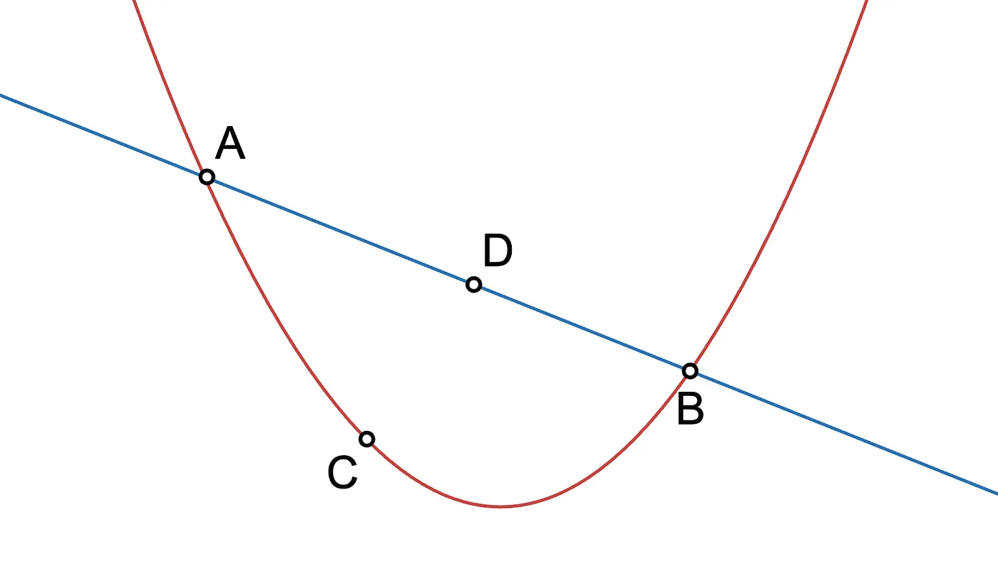
In the previous example, it is clear that interpolating three points yields a polynomial of at most degree two (a parabola), but it could also be of degree one if the points are aligned, or degree zero if they are aligned vertically.

This generalizes nicely to the following:

Interpolating $N$ points yields a polynomial of degree at most $N {-} 1$

Conversely, we need at least $N$ points to correctly encode a polynomial of degree $N {-} 1$. And this has the following amazing implication: if we take any univariate polynomial of degree $N {-} 1$, we can encode it by evaluating it at $N$ or more points. And then, anyone receiving those $N$ (or more) points could recalculate the original polynomial via interpolation!

So in a way, having a bunch of polynomial evaluations is an alternative way to represent some polynomial!

Now you should then be able to answer this very easily:

That’s all good and dandy — but how do we actually interpolate?

Lagrange Polynomials

Though there are faster ways to do this (via the Fast Fourier Transform), the canonical method is very clever, and it also provides some nice insights. So let’s look at that.

The idea is the following: suppose we have a set of $N$ evaluations. For a single one of those, let’s say $(x_i, y_i)$, we can build some special polynomial that will have a value of $0$ for all $x$ values except $x_i$, and exactly the value $1$ for $x_i$. Let’s call that polynomial $L_i(X)$.

It’s as if we were “selecting” $x_i$ mathematically using $L_i(X)$.

Why would we do this? Think of it this way: if we multiply such a polynomial by $y_i$, then we’ve just fabricated a small function such that:

$$f(x_i) = y_i L_i(x_i) = y_i"$$

Because $(x_i, y_i)$ is an evaluation of the original polynomial, what we want to get from the interpolation process is a polynomial $L(X)$ such that $L(x_i) = y_i$ for all our evaluations — so it seems $L_i(X)$ gets us halfway there.

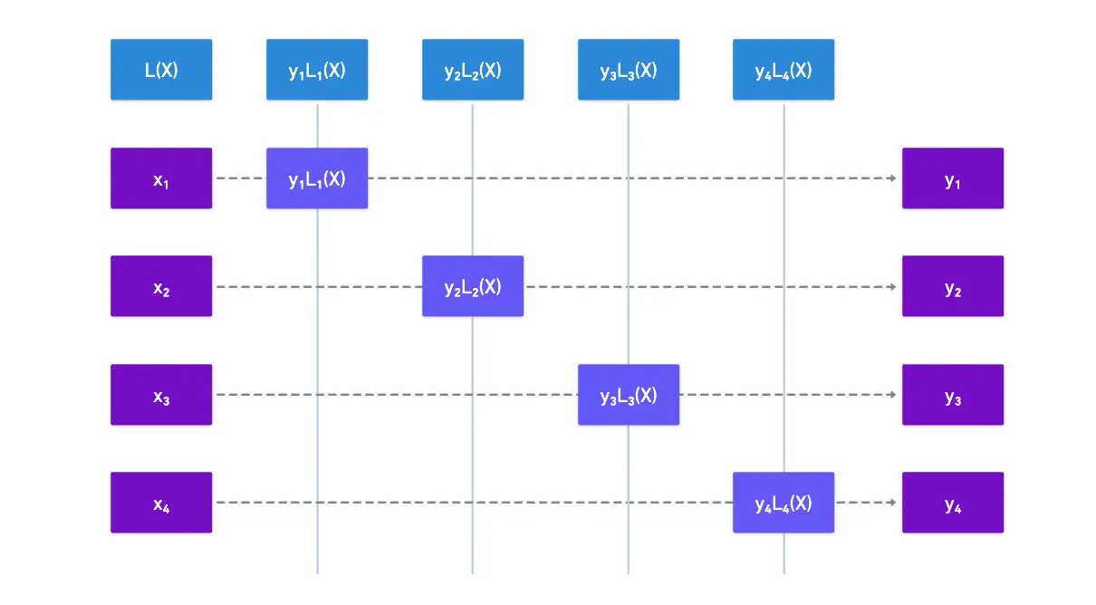
To get our interpolated polynomial, all we need to do is add up all values of $L_i$ for all our evaluations:

$$L(X) = \sum_{i=1}^{n} y_i L_i(X)"$$

And voilà! That will be the result of our interpolation. Visually:

Click to zoom

All that remains to nicely tie everything together is to determine how those $L_i(X)$ are defined.

Roots

Let’s recap our requirement real quick: each $L_i(X)$ needed to equal $1$ when evaluated on $x_i$, and $0$ on all the other evaluations.

A polynomial evaluating to $0$ is sort of a special occurrence. So much so, that we give these values a special name: any value $x$ such $P(x) = 0$ is called a root of the polynomial.

Despite their apparent simplicity, roots are very powerful. The main reason for this is the existence of an important theorem, called the Fundamental Theorem of Algebra.

As a general rule of thumb, when you see something called “fundamental” anything in maths, know it must be some seriously important stuff.

Simplifying a bit, one of the most important consequences of this theorem is that any univariate polynomial can be expressed as a product of linear factors:

$$P(X) = a(X {-} r_1)(X {-} r_2)...(X {-} r_n) = a\prod_{i=1}^{n}(X-r_i)"$$

A very important observation follows from this expression: a polynomial of degree $N$ has at most $N$ roots. This is such an important lemma that it doesn’t hurt to repeat it, for some dramatic flair:

A polynomial of degree $N$ has at most $N$ roots

This fact is extremely important, and results in some of the most powerful tools at our disposal. We’ll put this on hold for now though, but know that we’ll come back to this very soon.

Now, circling back to interpolation, it turns out this form is quite useful. It’s clear that when we evaluate any of those $r_i$ values, we’ll get $P(x_i) = 0$. We can use this to our advantage here: the $L_i(X)$ polynomials need to be $0$ on all $x$ values except $x_i$, which means they are roots of $L_i(X)$! Therefore, we can construct $L_i(X)$ as:

$$L_i(X) = a_i\prod_{\stackrel{j=1}{i \neq j}}^{n} (X {-} x_j)"$$

We’re intentionally omitting $x_i$ so that it’s not a root of the resulting polynomial.

Fantastic! The only detail we’re missing now is tuning that $a_i$ coefficient so that we get exactly $L_i(X) = y_i$. A simple normalization of the expression will do: take whichever value $L_i(X)$ produces at $x_i$, and divide the whole expression by that. This way, when evaluating $L_i(x_i)$, we simply get $1$.

The full expression is then:

$$L_i(X) = \frac{\prod_{i \neq j} (X {-} x_j)}{\prod_{i \neq j} (x_i {-} x_j)}"$$

And that’s pretty much it!

The set of these $L_i(X)$ guys is called a Lagrange basis. We might need to dig deeper into what this naming means later, but for now, the name should suffice for reference!

Summary

Alright! That’s gonna be it for today.

What we have for now may seem a little underwhelming. I mean, all we have are numbers and expressions — and these things probably feel a little basic.

Admittedly, there are a lot of layers of complexity to peel from these rather plain elements we’ve seen so far. But I don’t think it would be either practical or instructive to do so now.

Instead, it would be better to start exploring the applications that make use of these concepts. As we start using these tools, their potential will start becoming more apparent.

So on our next encounter, we’ll be looking at one of the simplest yet most fundamental protocols we can craft out of these building blocks presented today.

See you soon!