The ZK Chronicles: Circuits Revisited

In the previous article, we finally delivered on the promise of general verifiable computation. That is, the ability to feed in any program, and get a proof out.

As neat as it gets!

It's a pretty cool ability indeed, but let's not get carried away. That generality has a price tag, because we need to prove the correctness of the whole machine running the computation. Which means, in more concrete terms, having to deal with every fetched instruction, every register read, and every memory access, row after row of a gigantic trace.

Which begs a tiny question: if the computation we care about is small, and known in advance (something like perhaps a hash check, or a signature verification, or some business rule over private data), then... do we really need the full power of a virtual machine?

Obviously, I'm not giving all this prelude to say "oh no yeah we absolutely need the full machine" (although that would be a fun plot twist). Naturally, all this is to say that a circuit would do just fine, and it would be considerably cheaper.

Even the zkVM cases we discussed sidestep their problems with precompiles, remember? Which are nothing more than hand-written circuits, brought in to avoid paying the full price of the machine.

So here we are, vouching for circuits once again! The catch, of course, is that nobody in their right mind wants to write circuits by hand. We've been drawing these gate diagrams for quite a few articles now, but we never really said how to write gates! And I'm pretty sure we can all agree that writing every gate explicitly wouldn't scale anyway, beyond toy examples.

That doesn't mean we can't be smart about it, and avoid writing our circuits gate by gate!

So this time around, we'll start by looking at the middle ground: tools that let us write something that looks like a regular program, and turn it into a circuit for us. Doing so will take us through the journey from code to constraints, and into the proving system that does the heavy lifting afterwards.

And I'm sure you'll find the second part very satisfying, as it will make use of some very old acquaintances of ours!

That's more than enough preamble. Let's dig in!

Frontends and Backends

If you recall, we talked about the difference between frontends and backends way back when we discussed computation models. That distinction is a good place to start.

Tools for building ZK proofs from programs are usually split into two parts:

• The frontend is where we write our computation. It takes a human-friendly description and compiles it into some intermediate representation of a circuit (a set of constraints).
• The backend takes that representation, and runs a proving system on it: it generates (and then verifies) the proof.

Click to zoom

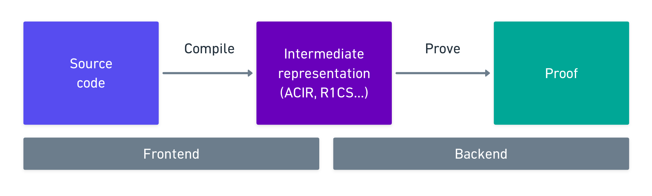
If you've ever seen how a regular compiler works, this should look very familiar. Source code gets lowered into an intermediate representation (like LLVM IR), which is then turned into machine code for some specific architecture.

The reason for splitting things up in the context of ZK is pretty much the same: specificity. The frontend's job is to define the ergonomics of writing our programs (or our circuits, but we'll see they look somewhat different in just a moment), while the backend decides how fast and small the proofs are.

That's the theory, at least! To make this more concrete then, let me introduce you to one of the biggest players in the modern ZK landscape.

Noir

Noir is a domain-specific language (DSL) for writing zero-knowledge programs, developed by Aztec Labs. Its syntax is heavily inspired by Rust, so describing a circuit feels a lot like writing a regular program.

On the architecture side, it's purely a frontend. It compiles our code into an intermediate representation, and leaves the proving to whichever backend we plug in.

Noir isn't the first of its kind, mind you. Circom is one of the oldest circuit languages out there, which compiles into R1CS, and is tied to its own toolchain. Noir, on the other hand, handles the conversion into an intermediate representation that any compatible backend can digest.

To see it in action, we'll use the same circuit we used back a few articles ago, with three inputs ($w_0$, $w_1$, $w_2$), and only five gates computing the rest. In Noir, this is just:

fn main(a: Field, b: Field, c: Field) -> pub Field {
    let w3 = a + b;
    let w4 = b * c;
    let w5 = a + w3;
    let w6 = w3 * w4;
    w5 + w6
}

That's it! As you can see, we didn't write any gates (nor selectors or tables for that matter). A Field is simply an element of the field our proof system works over, and the pub in the return type means the output is a public value.

By the way, everything here is a private input by default. That's the sensible choice for zero knowledge, so we can opt into making things public, and not the other way around.

The next step is to take this code and compile it, which you'd typically do using nargo (Noir's compiler), resulting in something like this:

private parameters: [w0, w1, w2]
public parameters: []
return values: [w3]
ASSERT w4 = w0 + w1
ASSERT w5 = w1*w2
ASSERT w3 = w4*w5 + 2*w0 + w1

That right there is the intermediate representation we've been talking about, called ACIR (Abstract Circuit Intermediate Representation).

Notice that there are three constraints instead of five! The reason for this has to do with a discussion we had back in our R1CS days: only multiplications really cost, and additions can be collapsed together.

The example we just saw is rather plain, so here's another one that shows how circuits differ from regular programs. In a circuit, we can't just skip part of a computation, so something as innocent as an if gets treated very differently. Take for instance this tiny function:

fn main(s: bool, v1: Field, v2: Field) -> pub Field {
    if s { v1 } else { v2 }
}

And this is what the compiler gives us:

BLACKBOX::RANGE input: w0, bits: 1
ASSERT w3 = w0*w1 - w0*w2 + w2

The first line makes sure that the condition $s$ is actually a bit. And the second one is just:

$$w_3 = s \cdot v_1 + (1 {-} s) \cdot v_2$$

If you've been paying attention, I bet that looks familiar!

And if you don't, it's alright! Not that I'm testing anybody here. It's all good!

The reason for that is that it's exactly the same switch formula we used for our toyVM! The trick that lets a zkVM choose between instructions is the one a compiler uses to turn an if into arithmetic: both branches are always there, and a selector decides which result to keep.

Not that surprising, if you think about it. An instruction set is just a big chain of ifs, after all!

Okay, that's enough Noir syntax for today. My goal here is not to get into much detail about the language specifically. If you want to learn it properly, the official documentation is a great place to start!

However, this little taste is enough to observe one thing: nothing in the ACIR says anything about how to build a proof out of it. Because we already know, that's the backend's job - and any backend that can understand this language could, in principle, create proofs out of it.

And that's where things get really interesting.

Exploring the Backend

The default backend for Noir is Barretenberg, which in turn defaults to a proving system called UltraHonk.

Which sounds in equal parts scary and funny, doesn't it?

Understanding UltraHonk will be our main goal for the remainder of today's article. In order to do it, we'll need to understand that it's really a modification of another proving system - one that we happen to know really well by this point: PLONK!

What's with the weird names anyway?

Still, I think a little recap won't hurt anyone (but feel free to skip it if you remember the details!).

PLONK Recap

Long story short, the central idea behind PLONK was that circuits get arranged into a table, each row representing a single gate, with columns for the wire values and for the selectors that say what each gate does. Then we saw that for this to make sense, every row must satisfy:

$$q_L \cdot a + q_R \cdot b + q_O \cdot c + q_M \cdot a \cdot b + q_C = 0$$

In addition, we require that wires that must carry equal values actually do so (the so-called copy constraints), and we impose this condition in the form of the running product argument.

Finally, each column is interpolated as a polynomial over the roots of unity, the constraints are bundled into a polynomial that must vanish over all those roots (which means being divisible by a vanishing polynomial), and a quotient polynomial is built to show it. And KZG openings at a random point tie everything together.

Wow, I'm amazed at how short that summary turned out! Of course, if you want more details, you can always refer to the full PLONK article.

It works wonderfully, but it's not perfect by any means. Some of its biggest problems include:

• Interpolating and computing the quotient polynomial requires FFTs over large domains, which is often the bottleneck for the prover in big circuits.
• The quotient polynomial's degree grows with the degree of our constraints. That hurts custom gates, which pack more work into a single row (think of an elliptic curve point addition), but at the price of higher-degree constraints.
• Roots of unity of order $n$ only exist in $\mathbb{F}_p$ when $n$ divides $p {-} 1$. Since FFTs (and our row-numbering) want $n$ to be a power of two, the field needs $2^k$ to divide $p {-} 1$, for a $k$ large enough to fit all our rows. That's a real restriction on the fields we can choose.

For example, the scalar field of BN254 has $2^{28} \mid p {-} 1$, which is plenty. But Mersenne31 has $p {-} 1 = 2 \cdot (2^{30} {-} 1)$, where the second factor is odd: the only power of two dividing it is $2$. That's the same obstacle we ran into in the exotic domains article, and it keeps us from using fields like that one.

Upon closer inspection though, we can see that most of these problems come from only a couple places, namely the FFTs and how constraints are checked.

Hm, interesting. An idea comes to mind then: couldn't we try keeping the "good" parts (the arithmetization and the copy constraints), and perhaps think of a different way to check those constraints?

The Swap

Well, that's easier said than done! It's not immediately clear what to try.

However, since the main problems had to do with roots of unity, then maybe a good place to start would be to change the way we number rows.

During our adventure together, we've seen at least one other method we can try, although it was a long time ago. So I'm just gonna say it. Ready?

Binary strings!Binary strings!

Yeah! If we have $N = 2^d$ rows, then each row is identified by a point $x \in \{0,1\}^d$, which is a vertex of the boolean hypercube.

And that opens up some interesting possibilities! Recalling our pass through multilinear extensions, we could take a list of numbers, index them with points in a boolean hypercube, and then encode them in a function, like so:

$$f(0,0) = 2 \quad f(0,1) = 3 \quad f(1,0) = 5 \quad f(1,1) = 8$$

The list being encoded here is $[2, 3, 5, 8]$.

But how does this help us? Well, if we focus on the columns of our table, we'll see each one of them is simply a list of numbers! Therefore, if we number the rows using our hypercube's vertices, then we can encode each column as a single multilinear extension!

If you think about it, this is not very different from how PLONK handles columns, which is through interpolation. But where interpolating gives us a univariate polynomial, this new strategy gives a multivariate polynomial $\tilde{P}$ in $d$ variables (with $d$ being the dimension of the required hypercube, so that we can encode every row as an element in $\{0,1\}^d$) that:

• Agrees with the column on the hypercube, so $\tilde{P}(x)$ is the entry at row $x$, for every vertex $x$.
• Extends beyond the hypercube, so we can also evaluate it at points whose coordinates are any field elements.

And among all the polynomials that do this, there's exactly one that's multilinear. For our little list, that would be:

$$\tilde{P}(X_1, X_2) = 2 + 3X_1 + X_2 + 2X_1X_2$$

That gives us an encoding strategy, but now we need to build checks around it. So what kind of checks do we need to make?

The Check

Just like in PLONK, every row has to satisfy the gate equation from the recap. So we should perhaps start by swapping each column for its MLE, meaning that $a$, $b$, $c$ and the selectors now denote polynomials in the $d$ variables. With that, the left-hand side of the gate equation becomes a polynomial too:

$$F(x) = q_L(x) \cdot a(x) + q_R(x) \cdot b(x) + q_O(x) \cdot c(x) + q_M(x) \cdot a(x) \cdot b(x) + q_C(x)$$

Notice that when evaluated at a vertex $x \in \{0,1\}^d$ of the hypercube, this gives us exactly the relation's value at row $x$. And that's how we'll write any relation from now on: $F$ is the polynomial expressing it, and the circuit is satisfied when, for every vertex $x \in \{0,1\}^d$, the relation holds. Meaning:

$$F(x) = 0 \qquad \text{for all } x \in \{0,1\}^d$$

All that remains is to prove that something is zero over all of the $2^d$ points. And we must do it in a way that's cheap for the verifier, so that we get an improvement over standard PLONK (which was the whole point of the swap).

Boolean hypercubes, and an evaluation that should yield a big $0$. Spidey senses are surely tickling. This sounds like a job for...

A sum-check!A sum-check!

Indeed! We could try proving:

$$\sum_x F(x) = 0$$

Only one little problem remains, as the terms could cancel each other out.

For instance, $F(x)$ could be $+5$ in one row and $-5$ in another, and the total would still be zero.

The fix is a sprinkle of the usual: randomness. We have the verifier send a random challenge $\kappa$, and we weigh each row $i$ by $\kappa^i$, where $i$ is the row's index. With this, the claim becomes:

$$\sum_{i = 0}^{N-1} \kappa^i \cdot F_i = 0$$

It's useful to view that sum as a polynomial in $\kappa$. If any $F_i$ is non-zero, then the whole thing is a non-zero polynomial of degree less than $N$, and by Schwartz-Zippel it has very few roots. That means a random $\kappa$ will almost surely not make it vanish by accident, and the equation can only hold if every single $F_i$ is zero.

And there's a little extra detail we need to account for. We know sum-checks deal with sums of a polynomial in the variables over the hypercube, while our weight $\kappa^i$ is a function of the row's index $i$, which we described as just an integer. Thus, we need to express it as a function of $x \in \{0,1\}^d$.

Luckily, it's pretty easy to do that, since a point in the hypercube behaves just like a binary number, meaning we can express it as:

$$i = \sum_j x_j 2^j$$

Then, we can simply write:

$$\kappa^i = \prod_{j} \left(\kappa^{2^j}\right)^{x_j} = \prod_{j} \kappa_j^{x_j}$$

Where $\kappa_j = \kappa^{2^j}$.

Wait... with $x_j$ sitting in an exponent, that's not a polynomial in $x$ at all! True, true, but we only really care about what happens when $x_j$ is $0$ or $1$, and at those points, the factor $\kappa_j^{x_j}$ can only ever take two values: $1$ when $x_j = 0$, and $\kappa_j$ when $x_j = 1$.

So here comes a big brain idea: we can swap that for any expression that gives the same two values! And there's a very convenient one:

$$(1 {-} x_j) + x_j \kappa_j$$

Which is $1$ at $x_j = 0$, $\kappa_j$ at $x_j = 1$, and is also linear in $x_j$. Making that swap in every factor, we get a genuine polynomial in $x$, which we'll call

$$\text{pow}_\kappa(x) = \prod_{j} \left( (1 {-} x_j) + x_j \kappa_j \right)$$

It's multilinear, and it matches $\kappa^i$ on every vertex of the hypercube. Or in other words, it's the multilinear extension of the list $[1, \kappa, \kappa^2, \ldots]$, which is just the kind of polynomial sum-check is happy to handle!

In Barretenberg's code, these are called the gate challenges: the prover draws a single challenge and squares it repeatedly to get the whole list, exactly like we just did with $\kappa_j = \kappa^{2^j}$.

Putting it all together, what we need to prove is

$$\sum_{x \in \{0,1\}^d} \text{pow}_\kappa(x) \cdot F(x) = 0$$

And we already know how to do that: with the sum-check protocol!

Sum-Check in Action

Even though we talked about sum-checks a long time ago, I don't think we need to go through the steps again. So I'm gonna go a little faster here, and instead, focus on what we gain from this strategy.

If you want to check this step by step though, I do recommend you give the sum-check article a quick look before continuing!

Let's start with the prover's work, which used to be a bottleneck. On each round, the prover sends a small univariate polynomial to the verifier. Then, one variable gets fixed to the verifier's challenge $u_0$.

What does that do to a column? Well, its polynomial $\tilde{P}(X_1, X_2, \ldots)$ turns into $\tilde{P}(u_0, X_2, \ldots)$, which has one less variable. So now, it's described by half as many values: one for each vertex $y$ of the smaller hypercube.

And we can get those from the old table. Remember that $\tilde{P}$ is linear in $X_1$, which means that its value at $u_0$ sits on the straight line through its values at $0$ and $1$:

$$\tilde{P}(u_0, y) = (1 {-} u_0) \cdot \tilde{P}(0, y) + u_0 \cdot \tilde{P}(1, y)$$

The consequence then is that rows that only differ in that first coordinate get blended together, and this cuts the table size exactly in half.

Which might be reminiscent (because it's the same trick) of the split $g = (1 {-} X_1) \, g_0 + X_1 \, g_1$ we saw back in multilinear extensions!

The same happens on every round, so each column's table of values halves in size each time! Adding it all up, the prover handles $N + N/2 + N/4 + \ldots$ entries, which is about $2N$. That's linear in the size of the table, and crucially, it does not have any FFTs nor quotient polynomials. Which was the whole point of the swap!

What about custom gates, which made the quotient polynomial's degree grow? Now, a higher-degree relation only makes each of those univariate polynomials a bit bigger. For UltraHonk, their degree is at most $7$, which is just a handful of coefficients per round.

And what about the choice of field? PLONK needed roots of unity, and with them a big power-of-two subgroup. But the vertices of a hypercube are just tuples of $0$s and $1$s, and those exist in any field. So that restriction is gone from the constraint-checking part of the system.

Sure, other pieces may still have requirements of their own, like KZG needing a pairing-friendly curve. But the sum-check couldn't care less!

And this is the heart of the idea: keep PLONK's table, but check it with a sum-check over the hypercube. That strategy is what's called Honk.

If the idea of "PLONK on the hypercube" rings a bell, it may be because of HyperPlonk, the paper that made it popular. Honk isn't exactly HyperPlonk though: one of the differences is how the permutation argument is handled. But the spirit is the same!

So after $d$ rounds, the verifier is left with a final claim about a point $u$, made up of all the challenges. To check it, they need the value of every column at $u$, so the prover sends those along.

Keep in mind that gates aren't the whole story, of course: we also need to check copy constraints and lookups.

The good news is that a sum-check doesn't care what a relation looks like, so both just slot in as more relations: copy constraints through the same running product we saw in PLONK, and lookups through LogUp. We'll skip the details, since we've covered both before!

And when we saw the sum-check protocol for the first time, we said this was an oracle query, which we now know is checked through commitments the prover sends beforehand, in this case to the multilinear extension of each column.

Hang on a second. Do we know how to work with commitments for multilinear extensions?

The Commitment Layer

Relax, relax. It's not that big of a deal. We're well-prepared to take on a little extra!

Right - we know how to work our way through KZG, which is what PLONK uses. But KZG is built for univariate polynomials, not multilinear ones!

That calls for a different mechanism, and the one that comes to the rescue here is a protocol called Gemini, whose core idea is quite elegant.

Here's how it goes: take a multilinear polynomial $\tilde{P}$ in $d$ variables, with $2^d$ values (evaluations) over the hypercube. We'll write those values as the coefficients of a univariate polynomial $A_0(X)$ of degree less than $2^d$, in a very specific order: ascending, where each vertex is read as a binary number with its first variable as the lowest digit, just like we did when weighing rows with $\kappa^i$.

Read that way, $(0,0)$, $(1,0)$, $(0,1)$, $(1,1)$ are the numbers $0$, $1$, $2$, $3$.

For our little column example from before, listed in this order, we get $[2, 5, 3, 8]$, and so:

$$A_0(X) = 2 + 5X + 3X^2 + 8X^3$$

Next, we'll split this $A_0$ polynomial into even and odd powers, such that:

$$A_0(X) = E(X^2) + X \cdot O(X^2)$$

Looks familiar, doesn't it? Yeah, it's the same even/odd split from the FFT, and the one used for folding in FRI!

In our example, that's $E(Y) = 2 + 3Y$ and $O(Y) = 5 + 8Y$. Notice that $E$ holds the entries where the first variable is $0$, namely $\tilde{P}(0,0) = 2$ and $\tilde{P}(0,1) = 3$. Meanwhile, $O$ holds the entries where it is $1$: $\tilde{P}(1,0) = 5$ and $\tilde{P}(1,1) = 8$. So all the even/odd split is really doing is separating the table by the value of the first variable.

Which is why we organized the coefficients the way we did!

In other words, we can express $E$ and $O$ in terms of $\tilde{P}$:

$$E(Y) = \tilde{P}(0,0) + \tilde{P}(0,1) \cdot Y \qquad O(Y) = \tilde{P}(1,0) + \tilde{P}(1,1) \cdot Y$$

Now, I know we talked about this like a million years ago, but let's try to recall what we did in the sum-check to fix the first variable to a challenge $u_0$. What we did was blend each pair of entries, using this expression:

$$\tilde{P}(u_0, y) = (1 {-} u_0) \cdot \tilde{P}(0, y) + u_0 \cdot \tilde{P}(1, y)$$

That's a statement about values, one for each $y$. But look at how $E$ and $O$ are built: their coefficients are exactly those values, sitting in the same positions. So, what happens if we blend the polynomials $E$ and $O$ instead? Each coefficient gets blended with its partner:

$$(1 {-} u_0) \cdot E(Y) + u_0 \cdot O(Y) = \big[ (1 {-} u_0) \tilde{P}(0,0) + u_0 \tilde{P}(1,0) \big] + \big[ (1 {-} u_0) \tilde{P}(0,1) + u_0 \tilde{P}(1,1) \big] \cdot Y$$

Take a look inside those brackets. Each one is the blend from before, for $y = 0$ and for $y = 1$ respectively, so they are simply $\tilde{P}(u_0, 0)$ and $\tilde{P}(u_0, 1)$! That is, blending $E$ and $O$ gives us a polynomial whose coefficients are the table of $\tilde{P}$ with the first variable already fixed. We call it:

$$A_1(Y) = (1 {-} u_0) \cdot E(Y) + u_0 \cdot O(Y)$$

And with our numbers, that's $A_1(Y) = (2 + 3u_0) + (3 + 5u_0)Y$.

Of course, this is a simple 2-variable example. More variables would just be more cumbersome to work with, but the idea is exactly the same!

We can repeat this process, splitting $A_1$ into its own $E_1$ and $O_1$, and blending them with the next coordinate $u_1$. In general, this can be expressed as:

$$A_{i+1}(X) = (1 {-} u_i) \cdot E_i(X) + u_i \cdot O_i(X)$$

In essence, this is the same kind of folding we saw in FRI, only now the random challenge is replaced by the coordinates of the evaluation point. Each fold halves the degree, and fixes one more variable of the multilinear polynomial. And after $d$ folds, what's left is a constant, which is exactly $\tilde{P}(u)$!

Now, remember what we're after: the prover claims that $\tilde{P}(u) = v$ for some value $v$, and we need to check that against a commitment to $\tilde{P}$. Notice that every fold uses a coordinate of $u$, which means the folded polynomials can't exist beforehand: the prover computes them at opening time, once $u$ is known.

The only thing committed up front is the column itself. But wait... isn't that a univariate polynomial? So surprise surprise, we're free to use KZG to commit to $A_0$!

Then, the prover computes all the folds, and commits to each folded polynomial $A_i$ (the verifier can't compute them on their own, since they don't know the values of $\tilde{P}$). And since these are also plain univariate polynomials, KZG does the job just fine! The last fold, $A_d$, is just the constant $v$ that the prover is claiming, so there's no need to commit to it: the prover simply sends it.

All that's left is for the verifier to be convinced that each $A_{i+1}$ was properly built from the previous one. If that's the case, then folding all the way down from the committed $A_0$ really ends at $v$. This is checked at a random point $r$: the prover opens each $A_i$ at $r$ and at $-r$ (since $E(r^2)$ and $O(r^2)$ can be recovered from those two), and the next fold $A_{i+1}$ at $r^2$. With those values, the verifier checks the relation:

$$2r \cdot A_{i+1}(r^2) = r(1 {-} u_i) \left( A_i(r) + A_i({-}r) \right) + u_i \left( A_i(r) {-} A_i({-}r) \right)$$

You can check this one by plugging in $A_i(\pm r) = E(r^2) \pm r \cdot O(r^2)$. It all falls into place!

We chain these checks from $A_0$ all the way down to $A_d = v$, and as a result, the verifier becomes convinced that $v$ really is $\tilde{P}(u)$.

This way, we've turned a multilinear evaluation claim into a bunch of univariate evaluation claims, at a few points. But there's one minor problem: we need to check them all! And we don't want to run a dozen KZG openings.

Fortunately, there's a second tool for that, called Shplonk. It lets us batch many opening claims, at many points and for many polynomials, into just one.

It works by taking the witness polynomials that KZG builds for each evaluation, and combines them into a single one using a random linear combination - in the same spirit as when we reduced evaluations in GKR, or when we batched constraints in PLONK: use some randomness to squash many checks into one.

Barretenberg fuses both steps into one protocol called Shplemini. The end result is one single KZG opening that closes the entire thing. And that means we keep the same assumptions as PLONK in this department, including KZG's trusted setup.

There's also an alternative, called Zeromorph, that builds multilinear commitments out of univariate KZG in another way. And Barretenberg supports IPA too, if you'd rather avoid the trusted setup altogether!

The Ultra in Honk

Right. After all that, we could very well end things here. But we still have a couple of loops to close, and since we're almost at the finish line (for the whole series), I'll ask you guys to endure just a little longer.

I mean, we should be pretty seasoned at this point, so I'm sure we can go the extra mile!

Because you see, so far, the system we've been describing is Honk, not UltraHonk (which we said Barretenberg runs by default). So then, where the heck does that "ultra" come from?

To keep it brief, the Ultra part refers to the arithmetization, much like Plonkish was for PLONK.

The reason to reach for a different arithmetization has to do with vanilla PLONK rows being tiny, with just a single addition or multiplication each. Real programs are full of things that are awkward to express that way, like range checks, hashes, or elliptic curve operations, as we've mentioned in other occasions before! And since the prover pays for every row, it would be very nice if we could pack more work onto each one of them.

That's exactly what Ultra does. It gives each row four wires instead of three, and adds lookups and custom gates for the heavy hitters. Each of them is just one more relation, switched on by its own selector on the rows that need it. There are nine relations in total, going from copy constraints to range checks and elliptic curve operations.

Why four wires instead of three, you may wonder? Well, the width of a row is really a design choice, with 3 and 4 being the usual picks: every extra wire makes the proof and the prover's work grow a bit, but gives gates more room to operate.

For instance, a three-wire gate can add two numbers into an output, $a + b = c$. With four wires, the same kind of gate can add three numbers at once: $a + b + c = d$. That means adding up a long list of values takes about half as many rows!

And that's pretty much it!

Zooming Out

Ok, time to decompress a bit. I reckon that was a lot of information! This should be a good time to take a step back, and see how everything fits together.

In short, we kept the table, and changed the way we check that said table is valid. And when putting it all together, the high-level steps are not too different from what we're accustomed to:

1. Commit to the witness. The prover commits to the wire columns, plus the helper polynomials that copy constraints and lookups need (like the running product $Z$ from PLONK).
2. Run sum-check. The verifier sends the gate challenge $\kappa$, and both parties run the sum-check over the weighted combination of all relations. At the end, the prover reveals the evaluation of every committed polynomial at the point $u$.
3. Prove the evaluations. Through Gemini, Shplonk, and one KZG opening, the prover shows that those claimed values are consistent with the commitments.

And everything is made non-interactive through the Fiat-Shamir transform: the verifier's challenges are replaced by hashes of the transcript, in the random oracle model.

Oh, and I've conveniently skipped one thing: getting zero knowledge to work is a little tricky, since the messages exchanged in sum-check depend on the witness. We won't go into the details, but I'll say that zero knowledge can be achieved through masking techniques.

And I think now is a good time to revisit the boundary we mentioned right at the beginning of this piece: when should we reach for a zkVM, and when for something like Noir? The truth is there's no universal answer, but we can come up with a reasonable rule of thumb:

• If the computation is small, fixed, and well-understood, writing a circuit (with the help of a nice frontend) will most likely give you the cheapest proofs. As a bonus, you get full control over what's public and what's private.
• If the computation is large, changing, or already written in a general-purpose language, the zkVM's flexibility makes the machine overhead a price worth paying.

And mind you, they're not mutually exclusive! Remember precompiles? Many real systems combine both: general programs run on the machine, with circuits taking care of the hot spots.

So circuits are far from being a thing of the past. A Noir program can even verify another proof inside of it, which allows us to use recursion.

And if you look back, quite a few old acquaintances made an appearance: multilinear extensions as the way to represent columns, sum-check as the engine checking all the constraints, polynomial commitments closing the oracle query we left open, folding in the form of Gemini, and LogUp as the perfect partner for sum-check.

What a comeback story for sum-checks and MLEs, huh?

Everything ends up connected!

Summary

And that's a wrap for today!

Inadvertently, we've reached somewhat of a milestone. From the very beginning of the series, we've been building towards this promise of general verifiable computation: proving the correct execution of any program, in zero knowledge. And now we can do it with a zkVM when we need generality, and with a circuit compiler when we want efficiency.

And we should now be more familiar with key concepts like what a frontend and a backend mean in the context of ZK. In today's case, Noir plays the role of the frontend, allowing us to write something that looks like a regular program, and lowers it into an intermediate representation, like ACIR.

From there, the backend takes over. We got a taste of Barretenberg's proving system, UltraHonk, which keeps PLONK's table but checks it with a sum-check over the boolean hypercube, instead of a quotient polynomial. And in doing so, it brought back a lot of the concepts we introduced early in the series, like multilinear extensions.

In a way, this is a testament to how simple ideas can pay off big time!

But the story doesn't end here. The theory can only take us so far, and for any of it to make sense, we must discuss one more thing: the applications that ZK technology may have.

So what better way to end our journey than to see how ZK is faring in the real world?

The next one will be our last stop, so I'm looking forward to seeing you there!