 arkana
The ZK Chronicles: SNARKs (Part 2)
We now look at a second technique to build SNARKs that aims to fix some of the shortcomings in our previous exploration.
Last time, we finally made it to our very first efficient zero knowledge protocol, in the form of Groth16. We called it a SNARK based on its characteristics: small proof size, fast to verify, and non-interactive.
But we were very cautious to always acknowledge the main pain point of the protocol: every single circuit requires its own trusted setup ceremony. If you change a single gate or add a single wire, you'll need to go through a full new ceremony: a complex and time-consuming multi-party ritual where you're relying on at least one participant being honest enough to destroy their fragment of the toxic waste. In a controlled environment, this may be tolerable. But in production, where developers may need to iterate on circuits regularly, this has the potential of becoming a serious bottleneck and also a serious security problem.
So we asked a question: can we do better?
The answer is yes. The construction that managed to do this, proposed in 2019 by Ariel Gabizon, Zachary Williamson, and Oana Ciobotaru, carries one of the most wonderfully tortured acronyms in all of cryptography: PLONK, which stands for Permutations over Lagrange-bases for Oecumenical Noninteractive arguments of Knowledge.
Yeah, I know. What the hell is "oecumenical" anyway?
Of course, this paper uses the Plonkish arithmetization technique we saw a couple articles back, so the publication managed to present not only one, but two amazing contributions to the ZK community.
Let's find out how they did it!
Current Limitations
Before we can appreciate what PLONK does differently, we may ask ourselves: can't Groth16 be modified to use a universal setup?
Understanding why this is not possible will give us some clues as to what we can do differently in this new argument system we're about to present.
Let's circle back to the proving key construction in Groth16 for a moment. For each wire in the circuit, the setup committed to a value of the form:
Those , , terms are the QAP polynomials we derived from the circuit's R1CS matrices, evaluated at the secret . Because gets discarded right after the setup, those evaluations need to be computed during the ceremony, with the circuit in hand.
And therein lies the root problem: we cannot recompute these polynomials after is discarded, so we circumvent this limitation by baking those evaluations directly into the structured reference string (SRS).
A quick analogy might help: it's like forging a custom key for a specific lock, then destroying the forge. The key is perfect for that lock and useless for every other one, and you somehow cannot build another copy of the key without the forge!

Ideally then, if we had a way to calculate these evaluations during proof generation and verification (implicitly, because is still toxic waste, but you get the point), then we may have what we need to find ourselves a universal setup.
PLONK achieves this by using an entirely different arithmetization, one whose polynomial structure doesn't depend on the circuit at ceremony time. The SRS becomes just a vanilla set of KZG powers:
Yeah, spoiler alert: we'll be using KZG!
Nothing circuit-specific in there. The ceremony happens once, and will support any circuit of a maximum size . The circuit description will live separately, as a set of public polynomials computed from the circuit and committed to using the SRS.
And we have already explored how the arithmetization that enables this looks like! So let's just go through a brief recap.
Plonkish Recap
Rather than encoding a circuit into three sparse matrices (as in R1CS), Plonkish organizes it as a dense execution trace table. Each row corresponds to a gate, and consists of exactly three wire columns: a left input , a right input , and an output .
| Gate # | Left input | Right input | Output |
|---|---|---|---|
| 1 | |||
| 2 | |||
| 3 | |||
| 4 | |||
| 5 |
One of the problems we immediately identified was that although we avoid the sparse matrices of R1CS, this table fails to capture the type of each gate. We can't tell whether we're looking at an addition or a multiplication gate by looking at the values alone.
To fix this, we introduced selector columns. These were a set of extra columns that live alongside the wire columns, and contain a handful of scalar selectors that determine what relation must hold between , , and for that specific row. And as a generalization, we defined this constraint template, which uses all those selectors:
By choosing the right selector values, we can express any standard gate. For instance:
| Gate type | |||||
|---|---|---|---|---|---|
| Addition | |||||
| Multiplication | |||||
| Constant |
It's just a plain and simple template, but it has enough expressivity to represent just about any circuit! I honestly find that quite beautiful.
And mind you, we're not limited to these five selectors. As I've already mentioned before, PLONK's descendants (TurboPlonk, UltraPlonk, Halo2) extend this idea with custom gates that encode complex operations in a single row. Just imagine if you could encode elliptic curve point addition (which would take dozens of R1CS constraints) into a single row here.
The possibilities are endless, but let's not get ahead of ourselves!
In the end though, this table is still just that: a table with values. To craft a proving system out of it, we're gonna need a few more things. And usually, the next step is to try speaking the language of polynomials!
So how do we do that?
Polynomial Encoding
Our strategy is gonna be to encode the question of whether an execution trace is valid into polynomial identities. As long as said polynomials satisfy certain relations, the execution is valid, and if they don't, then it's not. This reduction from circuit satisfiability to polynomial checks is what makes SNARKs possible.
And remember: there's always a subjacent language membership framing and the NP relation we talked about last time.
The idea is that the prover will have the full execution trace, which is our private witness , and they want to prove it corresponds to a valid execution. In this case, is the circuit description itself plus any public input the verifier knows about.
So what we're trying to do can be summarized cleanly as follows: we're trying to transform a set membership question , into a check around polynomial identities!
For this part of the story then, we're gonna need to tap into an old acquaintance of ours: the roots of unity. We'll use them to interpolate a few polynomials, and by doing so, we get a representation that's both FFT-friendly, and more importantly, independent of the circuit structure at setup time. This is what enables the universal setup: the SRS doesn't need to know anything about the circuit, because we're working in a generic evaluation domain that any circuit can use.
Let's see how. Suppose we have a circuit with a total of gates. To work with it, we'll pick the -th roots of unity as our evaluation domain. Using those as inputs, we can interpolate every column in our evaluation table, by assigning to each row an evaluation of the form . This will result in one polynomial of degree at most that passes through each of the values in a column.
So for example, will pass through the points for each row in the table.
Once we're done interpolating, we'll have a set of polynomials , , , , , , , . And what's nice about them is that they satisfy our gate constraint from before - so this becomes a polynomial identity that must hold at every :
It's important to note that these polynomials have different roles.
The wire polynomials , , encode the prover's private witness, so they change with every proof. However, the selector polynomials , , , , , are public parameters derived purely from the circuit structure. They're computed once during a preprocessing phase, and are the same for every execution of this circuit.
This separation is crucial: the selectors define what the circuit checks, while the wires contain what the prover claims!
At this point, we'll use a familiar trick: if this relation holds at every root of unity, then those are precisely the zeros or roots of the left-hand side polynomial. Which means the vanishing polynomial:
cleanly divides the polynomial from before, giving us a quotient polynomial :
Does this ring any bells?
It should, since it's the same divisibility trick we used in QAP relations! And we can use much the same reasoning from before: a valid execution trace will produce a left-hand side that's perfectly divisible by .
We'll see how this plays into the overall PLONK protocol later, but it's already looking pretty sharp.
Except, there's a catch.
Linking the Wires
Earlier, we mentioned the table representation is dense and efficient, but it has a massive structural gap: wire values will repeat across rows. When gates connect, the output of one feeds into inputs of others - and if a gate fans out (meaning the output is linked to multiple gates), that value appears in multiple places.
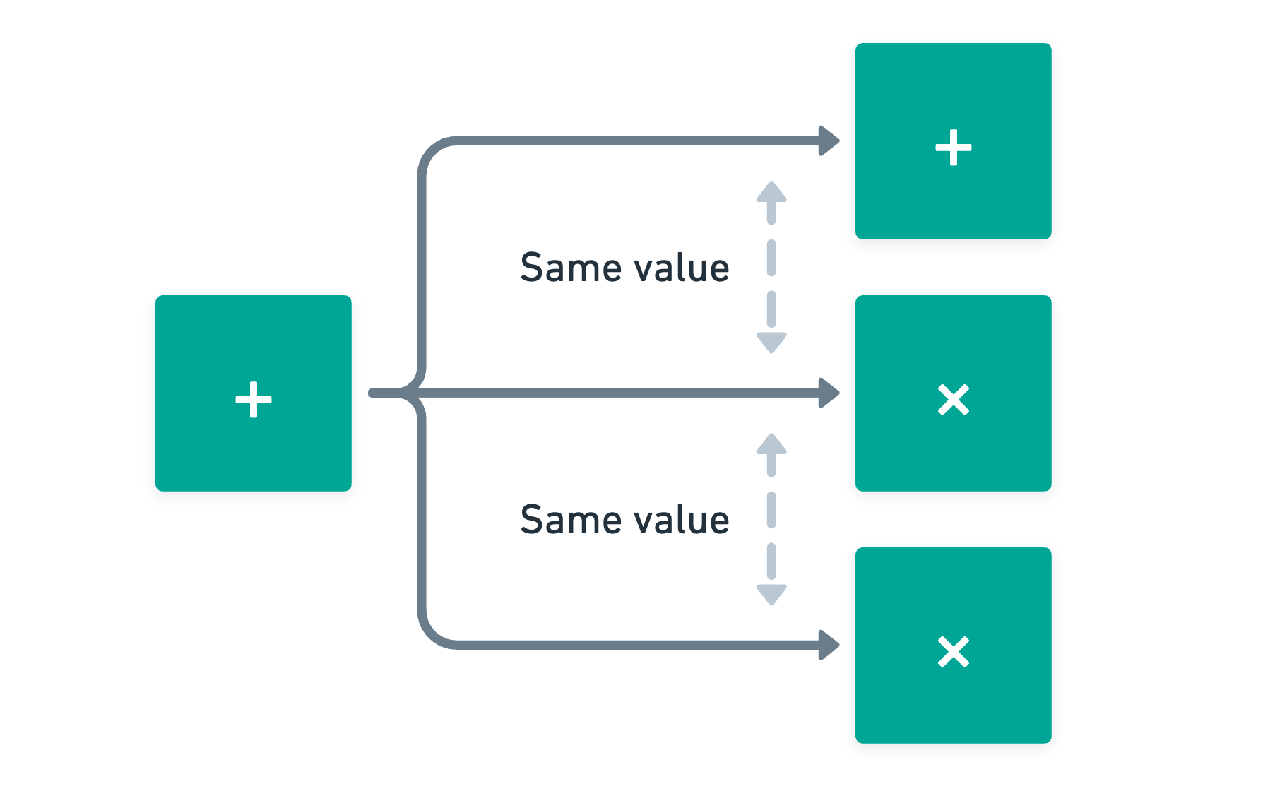
The problem is that each row verifies consistency for a single gate in isolation. Two table cells can hold different values for the same wire, and each gate constraint will pass all the same. The wiring is now implicit rather than structural.
If we don't take care of this limitation, it will completely break any further efforts, and so we need to introduce a new set of constraints, which we call copy constraints. Enforcing these is actually where PLONK's central construction is all about - and also where its funky name comes from.
Permutations to the Rescue
To represent the notion of "wire and wire hold the same value" in polynomial terms, we first need a way to access individual cell values. The standard way to do this is by assigning each cell in the table a unique label. With three columns and rows, that's labels total.
Note that these labels form their own space, distinct from our -th roots of unity!
Now, let's imagine for a second we have a polynomial that encodes every cell value at its label:
This gives us a clean framework to work with: cells that must hold equal values become a set of labels which should have matching evaluations. For instance:
Naively, we could check these equalities one by one. Alas, that scales linearly with circuit size. And since we're trying to build a SNARK here (which means small proof and fast verification), that's clearly a no-go.
So, is this a dead end?

Not at all! And actually, this is precisely where PLONK's magic pops into the scene: there's a neat trick to check all equalities in a set at once.
The trick is to use a permutation .
A what?
A permutation! It's just a little function with one simple job: to cycle through the labels in each constraint set. So if appears in cells , then creates the cycle :
Note that the permutations depend on the circuit structure, so they will also be calculated during a preprocessing phase for the circuit, and they will be public!
With permutations in hand, we can now make this fancy claim:
All copy constraints hold if and only if the multiset of values at original positions equals the multiset of values at permuted positions.

Here, here, don't panic. I got you.
A multiset is just a collection where duplicates matter. For example, {3, 3, 7} and {3, 7, 7} are different multisets. The claim simply says: if we collect all wire values and then collect them again after permuting labels, we get the same bag of values (with the same counts) , only if constrained cells truly hold equal values.
To build some intuition on how to check this (which will also lead us to the actual solution proposed in PLONK), let's take all labels in some set and compute the product of wire values:
Now, can you guess what happens when you apply the permutation?
Well, since just cycles through the set of labels, we get the exact same product!
Sadly, this alone is not enough. Upon closer inspection of those products, a question will probably come to mind: wouldn't this work for any set of wires, equal or not?
And you would be absolutely correct, it would! So to make this work only when the wire values are truly identical, we need one more ingredient. All we need to do is blend in the labels themselves:
That small patch makes it so that these products are equal if and only if all the values coincide. The key lies in that subtle discrepancy in the second product: the label doesn't match the input to . When values differ, this offset destroys the equality.
You can try this yourself with a small list of values, and any indexing strategy!
With this, we can confidently say that the multiset is no longer invariant under permutation, unless of course all values are actually the same.
And the cherry on top: we can check this equality efficiently!
The Running Product
Rather than computing both big products at once and comparing them, the prover will use a different strategy: they will build up the ratio incrementally using what we call a running product polynomial (sometimes called the grand product).
Think of as an accumulator: it tracks how the numerator and denominator balance as we walk through the table, row by row.
At this point, we need to stop thinking in terms of , and go back to our original trace polynomials , , and . We only needed to build some intuition, but the real wire encoding lives on those three polynomials.
Which means that at row , we have wire values , , . And we can start accumulating results one gate at a time, like this:
Where map each cell to its label in the label space, and encode the respective permutations. Again, these are all part of a preprocessing step!
Sure, that expression on its own doesn't balance out... but what happens once we've covered every single gate in the circuit?
What will happen is that once we reach , it will contain the contribution of every single gate in the numerator, and the corresponding permutation for each of those terms in the denominator. And if all the copy constraints do hold, then all those terms will cancel out in the end!
Thus, the prover (who is in charge of calculating ) will set , and then start an iterative procedure by processing one row at a time, obtaining the values for , , and so on. Each of those values will accumulate the ratio associated with the particular gate being processed, so upon reaching , we should get the full cancellation, meaning that !
Perhaps this is not so easy to see, so I'd like to propose a little exercise if you have the time: just go through our simple circuit example step by step! Seeing the cancellation in practice might help convince yourself that this does indeed work!
And that's the gist of it! Of course, we'd still need to transform this into a polynomial identity we can check. Before we do that though, I must let you into a little secret: there's a very subtle problem with this argument as we've defined it. We'll want to address it before we continue!
A Little Caveat
You see, this is a big product, after all. And there's a single number that doesn't get along too well with this notion of accumulating contributions: zero!
Zero would pretty much spell disaster. Think about it: what happens if some term in the product happens to equal zero? On the numerator, it would cause the whole product to be zero, but it would be an even more disastrous problem in the denominator, because we'd be dividing by zero!
Which of course, absolutely breaks the argument!

Luckily for us, this whole disaster can be easily avoided in a very simple way: just throw in some randomness into the mix!
Besides , we'll also ask the verifier to issue an extra random challenge , and we'll add that to each term in our product, so:
By doing this, we're offsetting each of those values by some random value, making it extremely unlikely for any of the terms in the product to equal zero.
Crisis successfully averted!
The Polynomial Identity
Lastly, what we need to do is build the polynomial identity to check for this permutation argument. So after the prover takes all the calculated values and interpolates the polynomial , there's a total of two polynomial identities we can build out of it.
The first one, we can call a step constraint: each step should match what we see in the running product. That means, if we reorganize a little:
Note that we use a property of the roots of unity there: is a clever way to obtain when !
The second identity is the boundary constraint, which is just to say that once we've gone through the steps, we should recover . But here, we can make a nice observation: since is a cyclic group, , so . That means the wrap-around condition and the initialization condition are the same thing! And so, a single constraint is enough:
Where is the Lagrange basis that equals at , and everywhere else in .
This is actually where the other part of the PLONK naming comes from!
This seeds , and the step constraint carries that forward through all rows. At the last row, the step constraint wraps around naturally because , closing the loop without needing any extra condition.
And there you have it: every copy constraint in the circuit, regardless of how many they are, is encoded into two polynomials and , and just two polynomial identities!
Quite elegant, right?
Batching the Checks
Before we assemble the full protocol, there's one more trick worth describing.
Right now, we have three separate polynomial identities the prover needs to prove: the gate constraints from earlier, and the brand new permutation constraint and boundary constraints .
Sure, we could handle these separately. But there's an even better approach: combine them into a single check, using what we call a random linear combination.
This is a trick similar to the one we saw in GKR!
For this, the verifier sends a random challenge , and the prover constructs a single quotient polynomial:
If you analyze all three conditions, they happen to share the same set of roots, . Therefore, adding , , and together (or any linear combination of them) results in a polynomial that preserves the original roots, so we can divide it by the same vanishing polynomial from earlier (), and obtain a quotient for the full system!
This works so well because if any of the individual constraints fails, then chances are that the polynomial won't be divisible by . That means if we evaluate at a random point, then there's an overwhelming probability (courtesy of the Schwartz-Zippel lemma) that the polynomial identity does not hold.
This is further supported by being a random challenge. If it wasn't, the prover could try to forge some value that makes the polynomial identity evaluation work, and we don't want that!
Batching saves both proof size and verification time: instead of checking three separate polynomial identities, we check just one.
I guess this is a good moment to step back and take a panoramic view of what we've achieved so far. We started with a circuit and an NP relation , and we've reduced the prover's claim that their execution trace is a valid witness for this circuit into a single batched polynomial identity that checks everything all at once, through a simple divisibility test.
It feels almost impossible, but the math works! And that's exactly the power of algebraic proof systems: we can reduce complex computational claims to elegant polynomial checks.
Putting It Together
Great! We basically have all the ingredients now, so it's time to assemble the proving system!
The first thing that happens is the preprocessing phase we've alluded to a few times throughout the article. The selector polynomials and the permutation polynomials are derived from the circuit structure, and committed to using the SRS. Importantly, the outputs of this phase are public parameters: they're not part of the witness, and crucially, anyone can compute them independently.
This means the prover, verifier, or any third party can do this preprocessing, since both the circuit description and the SRS are fully public.
In practice, this is done once and the results are distributed, but there's no trust required here, since the derivation is deterministic. This is also what makes the setup universal: any circuit can produce its own set of public parameters from the same SRS.
Once the preprocessing has been cleared, the prover proceeds to execute the circuit, and obtains a full execution trace. What they want to do next is to convince the verifier that both the gate and copy constraints hold.
The approach here is to enable the verifier to check the polynomial identities on their own. For this to happen, the prover will commit to a bunch of polynomials using KZG commitments, so that the verifier can query them at values of their choice.
Finally, something that feels straightforward!
This commit-challenge-open dance has a formal name: it's an instance of a Polynomial Interactive Oracle Proof (PIOP, or just IOP). The prover commits to polynomials as "oracles" the verifier can query at chosen points, the verifier issues random challenges, and the prover responds with openings backed by proofs. PLONK is, at its core, a PIOP - and it won't be the last one we'll see.
And so, we can at last present the interactive part of the protocol. It goes like this:
- Witness commitment: The prover interpolates , , from their execution trace, and commits to them using KZG: , , .
- Initiate the permutation argument: the verifier responds with random challenges and . The prover uses these to compute the accumulator polynomial and commits to it: .
- Compute the quotient: the verifier sends challenge . The prover uses it to batch the constraints (as we saw in the previous section) and compute the quotient polynomial , committing to it: .
- Polynomial queries: the verifier sends a random evaluation point . The prover opens all committed polynomials at (and at as well, for the consecutive-value check). KZG provides the opening proofs.
- Check polynomial identities: with the openings, the verifier reconstructs the polynomial identities at and checks they hold. By Schwartz-Zippel, if everything checks out at this random point, it means the full polynomial identities hold with overwhelming probability!
And that's it, really! Easy, right?

Yeah, I reckon it's not easy at all to clear all the hurdles in the way, but once we have all the pieces, putting them together doesn't feel that crazy of a task!
Overall, the process ends up being a bit more complex than Groth16. And I guess this begs an obvious question: is this really worth the extra trouble?
Pros and Cons
As always, there are some trade-offs to consider.
First of all, we now use a universal setup. This is one of PLONK's most important features, made possible by the selection of KZG as the polynomial commitment scheme of choice. We just need to run a single ceremony to derive the SRS, and every circuit out there is covered!
As long as the size of the circuit doesn't exceed the length of the SRS!
On this same account, we can talk about flexibility. This is the other big win of PLONK: we can extend the selector template to our liking, which can give rise to all sorts of optimizations. Systems like Halo2 have turned this extensibility in nothing short of an art form!
Then, we have proof size to discuss. Here, PLONK loses to Groth16: a typical PLONK proof will typically have around 15 elements, when we count all the commitments and opening proofs. This is still succinct by any reasonable measure. It's just that the compactness of Groth16 is pretty hard to beat.
And lastly, we have verification cost. On this front, Groth16 and PLONK are pretty close since they both need a small (constant) number of pairing computations. PLONK's verification is slightly more involved due to the permutation check, but it remains fast and independent of circuit size, which is our requirement.
In short: Groth16 wins on proof compactness, and PLONK wins on setup flexibility and convenience. Depending on the use-case, we might need to gravitate towards one of the two options.
You know... classic trade-offs!
Summary
And with that, we've covered most of PLONK!
I was gonna say "that's PLONK in a nutshell", but I think that would be rather hard-pressed, given the complexity and scope of this piece!
Building on the Plonkish arithmetization from a couple articles back, PLONK manages to provide a universal setup, valid for any circuit up to a given size.
The key insight is that the circuit description (selector polynomials and the permutations) stays outside the SRS. The ceremony and the SRS become an infrastructure layer rather than a per-circuit requirement.
I intentionally skipped a rigorous proof of zero knowledge and knowledge soundness. We also glossed over some of the finer details. These are crucial if we're implementing the protocol, but since we're trying to cover the core concepts, I think it's ok to skip that here!
As always, there's much more to say. The original PLONK paper is actually fairly approachable, and with the context you already have after reading this, it should be all the more accessible.
There's also the Halo2 book, an excellent resource for seeing how Plonkish gets used in practice.
PLONK and its descendants are the main workhorse powering ZK proving systems. More precisely, the Plonkish arithmetization (and its extensions) has become very popular. Which means that this is a solid foundation to understand the current ZK landscape!
Everything we built today hinges on a single tool doing its job: the KZG polynomial commitment scheme.
It requires pairing-friendly curves, and a trusted setup. It's definitely manageable, but...
What if we wanted to go fully transparent?
That's exactly the question STARKs were born to answer. So that will be our next stop!
Did you find this content useful?
Support Frank Mangone by sending a coffee. All proceeds go directly to the author.