The ZK Chronicles: zkVMs

Alright! It's been quite the journey so far, huh?

We've covered many interesting topics, spanning from the very basics of circuits, to the fancy terrain of recursive proofs from the previous delivery. And our focus has always been the same: to try and build proving mechanisms for specific computations.

In this regard, we've been mostly working off of the same premise, which is that we can design a circuit for whatever we want to prove. Knowledge of a hash preimage, satisfaction of a set of constraints, even correct calculations through lookups (which we then cleverly incorporate into our circuits), there's plenty we can cover. And in all of these cases, a lot of focus was placed on the careful and purpose-driven design of circuits.

To be fair, hand-crafting circuits is perfectly fine for many specialized cryptographic applications. However, most of the software running in machines around the world is not a custom circuit, but a program.

This whole series started with the claim that we'd be working with verifiable computing. And although we've put in a lot of effort so far, we would still be hard-pressed to say we're able to work with arbitrary programs.

If we manage to do that, however, I think we'd finally be able to get a well-rounded sense of completeness for this whole endeavor.

So how do we do that? How can we prove, say, that a smart contract was executed correctly, or that some piece of private computation was done as intended? How do we manage to prove the correct execution of any program?

This is the promise of a zkVM: a machine to which you feed any program and some input, and which produces a proof that the output is correct, with no need to specify any circuits.

But of course, this is easier said than done! Getting there will take some work - and as we'll see, the community hasn't fully converged on a single answer.

So let's see what we can do about it!

Programs

Let's start from the very top: what exactly is a program?

A program is nothing more than a sequence of instructions, belonging to a fixed set of possible instructions (an Instruction Set Architecture, or ISA for short), that are executed on a general-purpose processor. And if you're reading this on your mobile phone or your desktop computer, that processor is a CPU.

CPUs are, at their core, state machines. At any moment, they have a state: the values in the registers, the contents of memory, and a program counter pointing to the current instruction.

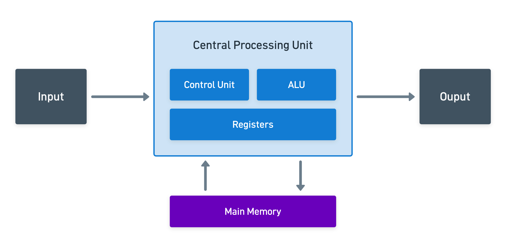
Diagram of the typical Von Neumann architecture

This state machine advances in a series of steps, which look like this:

Fetch the instruction at the program counter
Read the relevant register or memory values
Execute the instruction (add, XOR, load, store, branch, and others)
Write the result back to registers or memory
Advance the program counter

Because it's a state machine, we can collect the state of the CPU at every step, writing down every register value, every memory cell, and every program counter value, as if they were frames in a movie.

And if we put that on a table, what do we get? Yeah, exactly what you're thinking:

An execution trace!

That's our big brain moment right there: proving that a program ran correctly is equivalent to proving that this table is valid.

Golden sheet meme — Magnificent. Sublime.

To be specific, three things must hold:

Instruction correctness: the state at step $i+1$ is what you'd get by applying the instruction at step $i$ to the state at step $i$ .
Memory consistency: every memory read returns the value that was most recently written at that address.
Boundary conditions: the trace starts from the right initial state and ends at the claimed output.

Of these three, the first and third are essentially local properties, since each row can be checked against its immediate neighbors. But memory consistency is a different kind of beast: a read at step $i$ might refer to a write at a much later step $j$ , so it can't be verified row by row. It's sort of a global property of the entire trace.

To my knowledge, the standard approach is a permutation argument, constructed by sorting all memory accesses by address and timestamp, then checking that every read sees the most recent prior write at the same address.

It's an elegant but non-trivial piece of machinery that deserves much more attention than what I'm willing to give it in this article, so for now, we'll set it aside and focus on the instruction side of things!

These are all constraints placed on the trace, and we know how to work with them, at least in principle: arithmetize the trace, build a proof, and we're done!

A Tiny Example

Okay, I reckon all this nonsense is not that easy to digest. So how about we work through a small example, and actually see everything in action?

We'll build our very own toyVM. It will have just two registers $r_0$ and $r_1$ , and a grand total of three instructions:

$\texttt{SET } r_a \; v$ : load the constant $v$ into register $r_a$ .
$\texttt{ADD } r_a \; r_b$ : replace $r_a$ with $r_a + r_b$ .
$\texttt{MUL } r_a \; r_b$ : replace $r_a$ with $r_a \cdot r_b$ .

The one liberty we'll take is that all arithmetic will happen directly in our field $\mathbb{F}_p$ . Our registers will not be 64 bits long, and we'll have no overflow or any funny business.

Before you ask: yes, we're cheating. And we'll pay for this very soon, I promise.

Okay! Let's run a tiny program. How about computing $(3 + 4) \cdot 4$ ? It will go:

SET r0 3
SET r1 4
ADD r0 r1
MUL r0 r1

Now, remember what we said before: running this program is essentially the same as filling in a table. So let's do exactly that, writing down the state at every step:

step	$r_0$	$r_1$
0	0	0
1	3	0
2	3	4
3	7	4
4	28	4

This is the execution trace in the flesh, and as you can see, the final result sits on the first register in the very last row.

But a trace alone proves nothing. I mean, anyone can write a table with numbers. What matters is that these numbers carry meaning, and what makes them trustworthy is that every row follows from the previous one by correctly applying whatever instruction was active. That's the instruction correctness condition we mentioned earlier, and now we can finally pin it down.

Switching on a Constraint

The trick to this matter is to add a few extra columns, one per instruction, that act like switches: a $1$ if that instruction is the one running on this row, a $0$ otherwise. These should be familiar: they're the selectors from Plonkish arithmetization!

step	$r_0$	$r_1$	$s_{\texttt{set}}$	$s_{\texttt{add}}$	$s_{\texttt{mul}}$
0	0	0	1	0	0
1	3	0	1	0	0
2	3	4	0	1	0
3	7	4	0	0	1
4	28	4	0	0	0

For this to work, exactly one switch must be on per row (except for the last row, where there's nothing left to run). And with these switches in hand, we can write a single constraint that says " $r_0$ in the next row is whatever the active instruction says it should be":

r_0^{(i+1)} = s_{\texttt{set}} \cdot v_i + s_{\texttt{add}} \cdot (r_0^{(i)} + r_1^{(i)}) + s_{\texttt{mul}} \cdot (r_0^{(i)} \cdot r_1^{(i)}) + (1 {-} s_{\texttt{set}} {-} s_{\texttt{add}} {-} s_{\texttt{mul}}) \cdot r_0^{(i)}

I know the expression looks complex, but we can interpret it easily. Because only one switch is active at a time, all terms vanish except for one at any given row, leaving just the active instruction's update. Let's check the two interesting rows:

For row 2, where $\texttt{ADD}$ is on, the equation collapses to $r_0^{(3)} = r_0^{(2)} + r_1^{(2)} = 3 + 4 = 7$ .
For row 3, where $\texttt{MUL}$ is on, it collapses to $r_0^{(4)} = r_0^{(3)} \cdot r_1^{(3)} = 7 \cdot 4 = 28$ .

Like clockwork! One polynomial identity, checked across every adjacent pair of rows, certifies that the entire program executed correctly.

So that's the whole game, only in miniature: we model the machine as a state, lay its execution out as a trace, switch on the right constraint per row, and prove the table checks out.

And lest you think this toy is too much of a toy: the idea of a stripped-down machine built precisely to be provable is exactly how this whole field got started. The original was TinyRAM, a minimalist RISC machine with a mere handful of opcodes, that kicked off the entire zkVM line of research. Our toyVM is just a shrunken-down cousin of it.

Everything from here on is just about making this idea work in the context of a real CPU.

But that shouldn't be that different from what we've already done, right?

The Arithmetic of a CPU

Not so fast, cowboy.

We need to zoom in a little on those instruction constraints, to understand what they actually involve.

Take one of the very simplest cases: adding two registers. In most CPUs, registers have 64 bits of length, so that operation corresponds to $r_{\text{out}} = r_{\text{in},1} + r_{\text{in},2} \pmod{2^{64}}$ . It's a very simple operation in concept... until we remember our constraint systems live over prime fields $\mathbb{F}_p$ .

Modular arithmetic that's different from $\bmod p$ is quite a nuisance to represent, and as we already discussed in the past, it forces us to introduce range checks, carry handling, and overflow logic. In other words, we need several constraints just to represent a simple addition.

I know, I know - we already said this is usually best treated in terms of tables and lookups, but that strategy comes equipped with its own set of problems which we'll continue discussing further ahead.

And mind you, that's the easy instruction!

Things like 64-bit multiplication, bitwise $\textrm{XOR}$ , shifts, and comparisons all require their own set of constraints. And even if those are manageable, it's the sheer number of instructions to cover that becomes a real pain. Some manufacturers have even gone out of their way to introduce weirdly specific instructions over the years, that would make our life a nightmare.

So in summary, the constraint count adds up really, really fast. Plus, we have many CPU architectures to account for.

We could look in other places for some hope, such as Virtual Machines (VMs), but the story doesn't get much better even if we move to this territory. For example, the Ethereum Virtual Machine has its own instruction set, memory model, and semantics, and we might be tempted to think that could make things easier.

Teams like Polygon and Scroll spent years carefully crafting circuits for every single opcode (instruction) in the EVM. However, every time the EVM specification changes (and it does change over time), entire circuits could potentially be rendered stale, and need reworking.

This was a tremendous engineering effort, and is part of the reason why some chains have moved away from this model, like Polygon announcing their zkEVM project sunsetting in 2026.

So a natural question arises: what do we do to remove complexity?

Simplifying the Narrative

This is where one of today's protagonists comes in to save the day: RISC-V.

RISC-V is a clean, open architecture with roughly 40 base instructions, comprising additions, subtractions, bitwise AND/OR/XOR, shifts, comparisons, loads, and stores. That's just about it: it does not introduce any weird instructions, nor does it change over time.

And this is the fun part: most modern languages can compile to it. So what you can do is write normal code, and just compile it to RISC-V! Thus, our job is tremendously simplified: we just have to figure out how to build proving systems around computations compiled to this RISC-V architecture.

Hype aside though, using RISC-V architectures does not mean the cost of arithmetization disappears. At best, they just become more manageable.

On top of that, a typical program executes millions of instructions. Even at a modest, I don't know, 50 constraints per instruction maybe? That's tens of millions of constraints for a moderately complex computation, before even touching memory!

In short: proving CPU execution "naively" is very expensive.

As it turns out though, one of the biggest cost drivers isn't the gate count of individual constraints, but the tables those constraints need to reference.

And this is a problem we've already seen in the past, only with much, much bigger proportions.

The Large Table Problem

Proving that a result belongs to a list of possible results is the job of lookup arguments. The premise is much the same as before: if a value appears in a precommitted table of valid results, we've already covered at least half the story of proving such a value is a correct result. Everything from range checks, bitwise operations, and even CPU instructions can be expressed as lookups.

However, in past efforts we've assumed that the table we're working with is small enough to commit to. This was the case for a byte representation table, where we had 256 rows, and for something like a 16-bit $\textrm{XOR}$ table, which measures at 65,536 rows. Yeah, they are big (especially that second one), but they are still on a manageable scale.

But what about a real CPU?

Again, let's look at a simple addition: we'd need a table containing all possible $(a, b, a + b)$ triples, which would jump to a whopping $2^{128}$ rows! And as we'll see in a minute, committing to that table is straight up impossible.

This is commonly referred to as the large table problem, and it's one of the fundamental bottlenecks for lookup-based zkVMs.

Our direct lookup strategy from before will not cut it, so working with these gigantic tables calls for a different solution. So what can we do?

Table Decomposition

Let's try to imagine what we're after. The main problem we have happens during commitment: we need to use something like KZG or FRI, and those have costs that scale linearly with the number of rows to commit to. The $2^{128}$ possible combinations of an addition table means $2^{128}$ operations, which is straight up nuts.

You'd never finish computing so many operations.

Plus, in KZG, you also have to deal with the structured reference string (SRS), which also has size linear in the number of operations. No computer memory can deal with such a large SRS.

That being said though, not all tables are unmanageable - there's sort of a threshold on the size of tables we can efficiently work with.

Having said that, here's an idea: how about we try to break these large tables apart?

If we could split the tables into smaller, more manageable ones, then we could potentially commit to the chunks! But how do we do that? Do we just split them however we like? Does that even work?

Thankfully, we don't have to guess around, as there was a crucial paper that showed there's something we can actually exploit: structure!

Yeah! These tables may be large, but they aren't just random collections of triples: they have a certain regularity that we can tap into.

Lasso (the aforementioned paper) shows us that a large table of size $N$ can often be expressed as a combination of much smaller subtables, each of size roughly $N^{1/c}$ for some decomposition parameter $c$ . By doing this, the prover never has to commit to the big table, and instead they commit to the small subtables, where each lookup into the big table decomposes into $O(c)$ lookups into the smaller ones. As long as we can get to subtables of size $2^{16}$ or $2^{32}$ , we can manage just fine!

It's the same spirit from Bulletproofs and the FFT: instead of operating on an object of size $N$ , work on smaller pieces, and compose the results. Divide, conquer, fold - you know the drill!

Alright, that's a promising prospect for sure. But I guess the question remains: how? What does structure even mean?

The key insight here is actually pretty simple: for some functions, when you split their inputs into chunks, then sometimes you can compute the full output by processing every chunk almost independently from the others! That's what structure means, and under these conditions, a lookup into a big table is equivalent to several lookups into much smaller tables (one per chunk).

To see this in action, I guess the cleanest example is probably the $\textrm{XOR}$ table. A 64-bit $\textrm{XOR}$ has a full table with $2^{128}$ rows of $(a, b, a \oplus b)$ triples. However, $\textrm{XOR}$ acts independently on each bit, so we can split both inputs into eight-bit chunks:

\begin{gathered} a = a_7 | \cdots | a_0, \quad b = b_7 | \cdots | b_0 \\ a \oplus b = (a_7 \oplus b_7) | \cdots | (a_0 \oplus b_0) \end{gathered}

And that's about it! Because a single small subtable of $2^{16}$ rows covers all 8-bit $\textrm{XOR}$ results, the original 64-bit lookup decomposes into just 8 lookups into that subtable!

Addition is similar, but we need to be mindful of carry tracking between chunks. It's slightly messier, but the idea is much the same!

The Lookup Way

Of course, not every function out there has the sort of structure we're looking for. Hashes, for one, do not fit the Lasso paradigm at all.

But CPU instructions do. Which means that, if we're rigorous enough, we can express every single instruction of a CPU as a lookup! That's one way to build a zkVM then:

Represent each instruction as a lookup, and prove that each step of the trace belongs to one of the decomposed instruction tables

Jolt is one such example of a zkVM using lookups all the way down. I don't think we need to go any further into the details though, because we've already covered the fundamental intuition - so I'll leave that to your own curiosity!

This idea is very appealing from a theoretical standpoint.

If we take a moment to look back at the journey so far, it's amazing to see the entire paradigm shift we've been through. Early ZK proof systems (GKR, Groth16, PLONK) were all about arithmetic circuits, using them as their native computation model - but now we've seen that some systems, like these zkVM machines, are much better represented through other types of abstraction.

And the fun doesn't stop here: we also have to account for the millions of steps we said a computation can potentially have.

This is materialized in what's usually called continuations: execution is split into manageable chunks, which we can prove individually. And you can probably guess how this continues, if you recall the discussions from the previous article: we can fold the individual chunks together!

However, while Jolt is very sound and efficient in theory, it is not the most production-deployed system, at least not at the time of writing this article.

The Contenders

While the ideas behind Jolt were being matured, other research teams across the world were already working on their own zkVM solutions. But since they didn't have the theory behind Lasso, they had to make do with other tools and ideas.

In particular, you may wonder how they managed to deal with large tables. Well, this one might surprise you: they used STARKs!

And in hindsight, this abstraction also makes perfect sense. Think about it: didn't we say that the execution of consecutive instructions gives us an execution trace? And the action of "executing an instruction" itself could be represented as a state transition function, right?

Conceptually, at least!

Indeed, other players pushed this idea to its limits, with two of them emerging as the clear leaders in the zkVM space: SP1, and Risc Zero. So let's briefly talk about them, and see what choices they made!

SP1

SP1 is the zkVM solution developed and maintained by Succinct Labs, and it's probably the most widely adopted zkVM at the time of writing this. The central idea is quite simple: if execution traces are just very structured tables, then STARKs (which were literally designed around that idea) are the natural fit.

To make that work, SP1 is built on top of a STARK-based proving stack called Plonky3, which is a modern and highly-optimized library for building STARK proof systems.

Thus, the core plan is pretty much what you'd expect at this point: arithmetize the RISC-V execution trace using AIR, where each row of the trace represents one instruction step, and the constraints encode what a valid state transition looks like for each instruction type.

So yeah, we don't have to look up each instruction result in a table. But then, we need to solve another problem: how do we encode that state transition function?

The answer is exactly the switches from our toyVM, now at full scale: selector columns that activate the right constraint for each step, with only one "on" per row.

For instance, an $\textrm{ADD}$ instruction activates the constraint $r_{\text{out}} = r_{\text{in},1} + r_{\text{in},2} \pmod{2^{32}}$ , while an $\textrm{XOR}$ activates $r_{\text{out}} = r_{\text{in},1} \oplus r_{\text{in},2}$ - the selector matching the current opcode picks which one.

Encoding these constraints is fundamentally the job of Plonky3. And it's also what makes SP1 shine, thanks to its precompiles: for expensive, commonly-used operations (SHA-256, Keccak, elliptic curve arithmetic), SP1 replaces the full RISC-V execution with a hand-optimized circuit. Think of it this way: instead of proving the hundreds of individual steps for a SHA-256 call, a single precompile handles it in one shot. This gives enormous speedups on real-world workloads.

For long executions, SP1 uses the continuations trick, sharding the trace into fixed-size chunks, proving each shard independently, and then using recursive proof composition to collapse all proofs into a single one.

And if that wasn't enough, SP1 offers the ability to wrap the final STARK proof as a different type of proof. Meaning you can build, for example, a Groth16 proof for very cheap verification.

All in all, SP1 follows the same principle we've seen and talked about before: when the general solution is too expensive, specialize! Hand-craft the expensive parts, and let the general machinery handle the rest.

Risc Zero

Risc Zero actually predates SP1, and deserves a special mention for one reason: it was one of the first teams to demonstrate that a production RISC-V zkVM was feasible at all. Before Risc Zero, this was still largely theoretical territory.

While the architecture is very similar to SP1's (a RISC-V execution trace, AIR arithmetization, FRI-based polynomial commitments, and a Groth16 wrapper for cheap verification), one of the key contributions of Risc Zero was the idea of continuations, which as we've already seen, is quite ubiquitous in other zkVM systems.

By the way, the term comes from programming language theory: a continuation is just "the rest of the computation" from a given point onward. Here, it means that the output state of segment $i$ becomes the input state of segment $i+1$ , stitched together by the recursive proof.

Looking at the big picture, SP1 and Risc Zero are quite similar in architecture. The gap between them is less about fundamental design choices and more about execution: SP1's more modern backend and more importantly its extensive precompile library have given it a meaningful performance edge, and that's what's driven ecosystem adoption.

Which is a good reminder that in engineering, being right about the idea is only half the battle.

Morty soldering while Rick watches from the garage door — It's just how it is

Summary

Oof! That was a mouthful, eh? But we managed to cover a lot of ground today.

Everything started from the observation that, while well-intentioned and useful in the right context, circuits simply don't scale to general-purpose computation. And since the world runs on programs, and not circuits, applying ZK to general computation means we need to look for alternative ways to handle programs too.

That's where zkVMs come in. The idea behind them is simple in concept: to record the full execution as a trace, express the validity of that trace as a constraint system, and then prove the trace is valid.

Which makes sense because CPUs are state machines, with a set of valid operations that we can deal with in at least two different ways. Lasso uses lookup arguments, with all the table decomposition shenanigans that entails, and systems like SP1 and Risc Zero stick closer to the state machine premise, using STARKs and their state transition function approach.

And for long programs, continuations and folding close the loop: split execution into chunks, prove them independently, collapse everything into a single proof, profit.

With that, we've reached something of a milestone.

If you recall from the very beginning of the series, we've been building towards this promise of general verifiable computation: to prove the correct execution of any program, in zero knowledge.

And now we're here!

The story doesn't end here though, because we can only go so far with the theory. For any of it to make sense, we must discuss one more thing, which is the applications that ZK technology may have.

So what better way to end our journey than to talk about how ZK is faring in the real world!

The next one will be our last stop, so I'm looking forward to seeing you there!