Elliptic Curves In-Depth (Part 4)

We’ve covered quite a few things up until now, so I believe a quick refresher will prove to be helpful.

• The series started with a look at elliptic curves over $\mathbb{R}^2$ — what we now call affine space. The curves defined over this space are called affine curves.
• We then introduced an operation over these curves, baptized point addition. And we required precision, so we moved to curves defined over finite fields.
• Lastly, we explored the group structure of elliptic curves, induced by the point addition operation we defined earlier.

It would be completely fine if the series ended here. It’s possible to craft very useful algorithms with the knowledge we’ve acquired so far. No need to go deeper into the rabbit hole.

But if you’ve come this far, you probably want more. And much more to know there is, indeed.

Our journey continues with functions. This will unlock very interesting and powerful possibilities. Onwards we go!

Functions

Even though most of you will probably know what a function is, I think it’s worth giving a definition anyway. A function or map is like a box that takes an input, and returns an output. And it does so in a deterministic way: every time we pass the same input through the function, we get exactly the same output — no surprises.

Click to zoom

There are of course more rigorous definitions out there, but we need not linger on the details too much now.

When we think of a function, we usually imagine something like $f(x) = x^2$. Here, $x$ represents the input, and the calculated $x^2$ is the output. And more often than not, we picture these values as numbers.

But they need not be numbers!

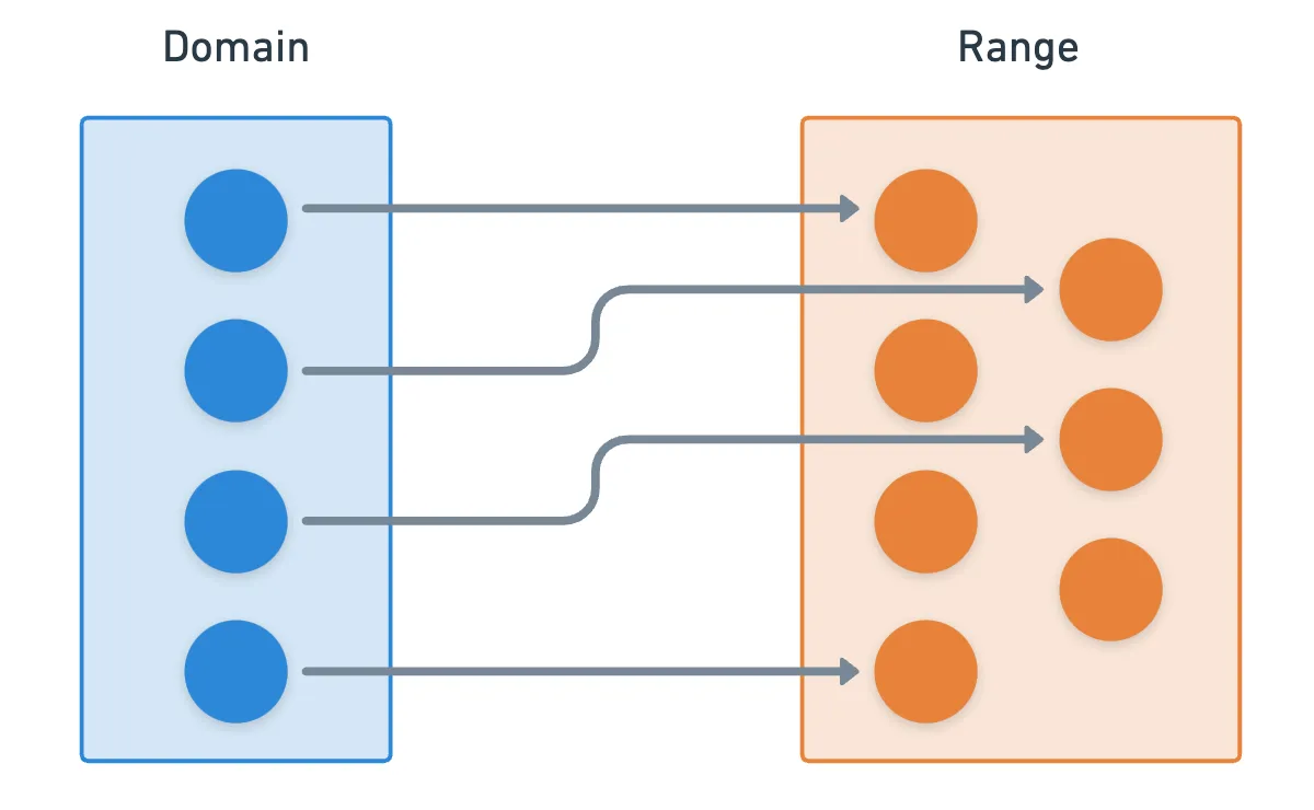
Inputs can belong to any set, called the domain of the function, and the outputs belong to another set, called its range (or sometimes also called the codomain).

Functions are also called maps, because of how they map each input in the domain to a value in the range.

So, how about instead of numbers, we try using groups as those sets?

Maps on Groups

Groups, as we already know, are structures resulting from the combination of a set and a binary operation. There are clever ways to define different maps that involve groups, using only this knowledge.

For example, one very simple relation would be the following:

$$f: \mathbb{Z}_+ \rightarrow \mathbb{G} \ / \ f(x) = [x]G$$

This is a function that maps every single positive integer to an elliptic curve group element.

Granted, if the group is finite, then some integers will have the same functional value. Formally, this means the function is not injective: a function is injective if each element in the domain maps to a unique element in the range. We’ll circle back to this in just a minute.

Click to zoom

Let’s take it a step further. Nothing really stops us from having a function where both the domain and range are groups.

There’s nothing very special about this. A function from some group $G$ into another group $H$ just maps each element of $G$ into $H$, and there could be a myriad of such relations. But what if we somehow managed to preserve some important properties?

Let me be a little more precise. If the group $\mathbb{G}$ has some operation denoted by $\cdot$, and $\mathbb{H}$ has another operation $*$, wouldn’t it be cool if a map between $\mathbb{G}$ and $\mathbb{H}$ could maintain some sort of relationship between these operations?

The operations need not be different, really. But in the more general case, they will be.

This leads us to one of the most important concepts in group theory: homomorphisms. A homomorphism is a function that preserves the group structure. What this means is that for any two elements $a$ and $b$ in $\mathbb{G}$, we have:

$$f(a \cdot b) = f(a) * f(b)$$

This might seem rather uninspiring, but it’s actually an incredibly powerful property. When working with homomorphisms, the order of operations doesn’t matter: we can either combine elements and then apply the function, or apply the function to each element and then combine them.

For example, the very first function I provided as an example happens to be a homomorphism.

Again, we’ll come back to this idea further down. For now, we’re just stockpiling on important definitions. Bear with me for a moment, please!

Isomorphisms

A couple paragraphs ago, we talked about injective functions. There’s another similar property of functions which we also need to understand, called surjectivity.

Click to zoom

Surjectivity alone is not that appealing (although it can be a useful in the right context). Things get really interesting when we combine injectivity and surjectivity.

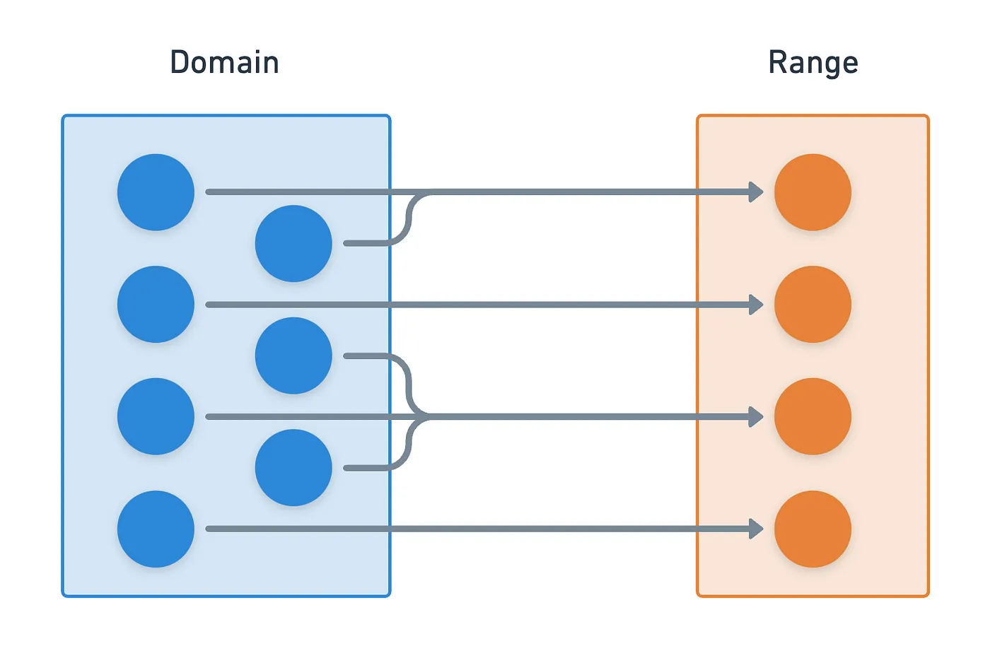
In plain english: injectivity guarantees that every element of the domain maps to a unique element in the range, and surjectivity guarantees that there are no unused elements in the range. This leads to something fantastic: a one-to-one correspondence. This is normally called a bijection.

Furthermore, when a homomorphism happens to be a bijection, it receives a special name: an isomorphism. It’s a one-to-one correspondence that also preserves the group structure — a “perfect” correspondence, so to speak.

When an isomorphism exists between two groups (we say that they are isomorphic), what really happens is that they are the same group in disguise. If you know what happens in one group, you automatically know what happens in the other one — the isomorphism gives you a way to translate results from one group to another.

Fact: every cyclic group of order $q$ is isomorphic to the additive group of integers modulo $q$.

Now we’re talking. This tool is actually quite interesting. Let’s look at a simple example. Consider these two curves over $mathbb{F}_{17}$:

• $E_1: y^2 = x^3 + 2x + 1$
• $E_2: y^2 = x^3 + 15x + 4$

At first glance, these curves look clearly different. Now, check this simple function:

$$f: E_1 \rightarrow E_2 \ / \ f(x,y) = (2x, 13y)$$

We first want to verify that, for any point $(x, y)$ that satisfies $E_1$, we get a point that belongs to $E_2$ after applying $f$. This is pretty straightforward:

• First, we substitute $(2x, 13y)$ into E₂. This yields $4y^2 = 4x^3 + 8x + 4$, after reduction modulo $17$.
• Now we multiply everything by the modular inverse of $4$, which is $13$ in $mathbb{F}_{17}$. After simplification modulo $17$, we obtain $y^2 = x^3 + 2x + 1$.

That’s exactly the expression for $E_1$! This is great — it means that the points $(2x, 13y)$ really satisfy $E_2$, because we arrive at an equality we know to be valid.

Next, we need to check that $f$ is indeed an isomorphism. Checking that it’s both injective and surjective is easy — I’ll leave it as an exercise to you!

About preserving the group structure, let’s just say that $f$ behaves nicely with the group law. We might go into further detail in future articles.

So there you have it! Two apparently different curves that happen to be isomorphic — thus behaving like the same curve.

From our previous example, an interesting question raises quite naturally, especially in the context of curves over finite fields: can we always find isomorphisms between curves?

Clearly, there’s something to be said about the group order. Two groups with different sizes cannot be isomorphic, for a homomorphism between them would either not be injective, or not be surjective.

But even when we have two curves of the same order, they may not be isomorphic. How do we evaluate this? Enter the j-invariant.

The j-invariant

The j-invariant has a fascinating history rooted in complex analysis, which is perhaps too deep of a rabbit hole for us to jump into right now.

Crucially, the key insight is that the j-invariant captures the essential shape of an elliptic curve. Two curves might look different at first glance, but if they have the same j-invariant, they’re really just the same curve (over an isomorphism, of course).

For a curve in Weierstrass form ($y^2 = x^3 + ax + b$), the j-invariant is calculated as:

$$j = 1728.\frac{4a^3}{4a^3 + 27b^2}$$

Yeah, I know. This formula seems to come very much out of nowhere. But it’s actually a distillation of a couple centuries of deep mathematics into a single expression.

We might go deeper into this topic later on. Hopefully. For now, just think of the j-invariant as a fingerprint for elliptic curves — each essentially different curve has its own unique j-invariant.

It’s all good and dandy with the j-invariant. Two curves that share this same characteristic value will indeed be isomorphic, but that’s just part of the story. What I didn’t mention is where those isomorphic curves are defined over.

Let me explain. Two curves might share the same j-invariant, but when we try finding an isomorphism between them, we may be unable to find it. No matter what we add or multiply the coordinates of points with, finding an isomorphism may prove an impossibly elusive task.

That is, if we restrict ourselves to finite fields as we know them so far.

Field Extensions

We’ve been working with finite fields like $\mathbb{F}_p$. Sometimes, these fields aren’t “big enough” for us to find those pesky isomorphisms we’re after.

Just like we can extend the real numbers to the complex numbers simply by adding $i$ into the mix, we can also extend finite fields by adding new elements.

For example, take $\mathbb{F}_{17}$. Suppose we wanted to find the square root of $2$ in this field — this is, a number that satisfies $x^2 \equiv 2 (\textrm{mod} \ 17)$. You can easily check that no element in $\mathbb{F}_{17}$ satisfies this relation.

But we can create a larger field that contains such an element. If we add an element $i$ such that $^2² + 1 = 0$, then a solution appears kinda magically. The numbers $7i$ and $-7i$ are the square roots of $2$. You can check this yourself.

In this context, we call $\mathbb{F}_{17}$ the base field, and the new field with $i$ is called a field extension. In this case, it’s written as ${\mathbb{F}_{17}}^2$.

It contains all elements of $\mathbb{F}_{17}$, plus new ones — a total of $17^2 = 289$ elements, to be precise.

It’s really like the complex extension of $\mathbb{F}_{17}$. But we’re not limited to defining $i$ in the way we did before, meaning that there are infinitely many possible field extensions!

Over these field extensions, we can now find those slippery isomorphisms prophesied by the j-invariant. Which brings us to our next topic...

Twists

When two curves are isomorphic when viewed over some larger field (a field extension), we say these curves are twists of each other.

The most common type of twist is called a quadratic twist. These are very easy to construct: you just multiply the $y^2$ term by a non-square $d$ (aka a number that doesn’t have a square root in the field):

$$E': dy^2 = x^3 + ax + b$$

Notice that this new curve has the same j-invariant of the original curve $E$. Therefore, an isomorphism between $E$ and $E’$ should exist — but the fact that $d$ is not a square makes it impossible to find over the base field.

As a sidenote, if $d$ is a square, then the curves are isomorphic over the base field!

This might seem nothing more than a curiosity, but twists are actually quite an important tool in cryptography.

In certain situations, we might find ourselves in the need of performing elliptic curve computations over field extensions. These are expensive (computationally) when compared to operations over the base field. And in cryptography, speed sells.

If you can find a twist of the curve that can operate over the base field, you can perform calculations there, and then map back to the original curve (group) via their connecting isomorphism. Pretty nice!

This is especially useful when dealing with Pairings. We’ll talk about them later in the series.

But it’s not as simple as it sounds. Nothing ever is. Finding such a twist might not be an easy task. Furthermore, we might stumble upon a weak twist — a group whose structure is easy to crack. This is why we often also require curves to have “secure twists”. An attacker who can’t break your curve might try to move onto a weaker twist, in the hopes of breaking your security. So I guess the existence of twists is kind of a blessing, and a curse!

Isogenies

Phew, we’re pretty deep into this already!

We’ve already talked about isomorphisms between curves — bijective maps that preserve the group structure. For some applications, they are exactly what we need. But sometimes, we might not need the full force of a perfect correspondence.

Maybe something slightly more flexible is just about enough. Perhaps an homomorphism — but just about any homomorphism? Other than trying to preserve the group structure, are there other properties we might want? This is where isogenies come into play.

An isogeny is a rational map between elliptic curves, that’s also a group homomorphism.

Let’s not worry too much about the rational map part, and let’s express this idea in simple terms. Apart from preserving the group structure, isogenies have another remarkable property: they preserve the identity element ($\mathcal{O}$). This means that they map the $\mathcal{O}$ in the domain to the $\mathcal{O}$ in the range (both being elliptic curve groups).

The simplest example of an isogeny is the multiplication-by-n map, $P \mapsto [n]P$. You can directly verify that the identity preservation condition holds!

Actually, this map leads to the concept of r-torsion points: points $P$ such that $[r]P = \mathcal{O}$. The set of all r-torsion points forms a group, denoted $E[r]$. We’ll talk about this in upcoming posts.

When put together, these two conditions also ensure something else happens: the kernel of an isogeny must be finite. The kernel of an homomorphism $f: E_1 \rightarrow E_2$ is simply the set of all inputs that map to the identity element $\mathcal{O}$ in $E_2$. It’s the analogous concept to roots.

For reference and rigorous proofs, I suggest checking out Hartshorne’s Algebraic Geometry, Chapter II. Proposition 6.8 shows proof of this. And I’m willing to bet that this is much more than what you bargained for when you started reading this.

Also if you feel especially adventurous, I suggest reading this.

In plain english: an isogeny can only collapse a finite number of points to $\mathcal{O}$. Or said differently, only a finite number of points can map to $\mathcal{O}$.

This is a very, very deep subject. To be fair, this just barely scratches the surface of what there’s to know, and most textbooks in this area are very technical and heavy.

And I still have a lot to learn myself.

What I’ll say is that isogenies have many applications in cryptography. One of the most interesting (and recent) applications relates to the difficulty of finding isogenies between curves.

Oh, because isogenies can be composed, leading to the concept of isogeny graphs. In fact, the difficulty of computing isogenies resembles finding a “hidden path” in an isogeny graph.

Some isogeny-based methods were even proposed as possible candidates for Post-Quantum Cryptography (PQC) algorithms — one such example is the Supersingular Isogeny Diffie-Hellman Key Exchange. Sadly, the method was recently cracked — but it was due to the specific structure of the scheme.

I reckon this section is quite simplified, but really, there’s so much to cover that we’d probably need a dedicated article!

Before we go, one more thing.

The Endomorphism Ring

Lastly, I want to talk about something we’ll come back to in a few articles.

There are many possible functions from $E$ to itself. One such example was the multiplication-by-m map (which is also an isogeny). We call such functions endomorphisms. Note that isogenies belong to this category.

Shifting our focus to the maps themselves reveals something amazing: they have a ring structure. Adding together two endomorphisms results in another endomorphism, and multiplication is just composition of these maps (also resulting in an endomorphism).

The ring is usually denoted $\textrm{End}(E)$.

One example of an endomorphism that’s quite different from our trusty multiplication-by-m map is the the Frobenius endomorphism, defined as:

$$\pi: E \rightarrow E \ / \ (x,y) \mapsto (x^p, y^p)$$

Essentially, it just grabs the coordinates of a point, and raises them to the power of $p$ — the size of the finite field. Doing this has a nice property: the map acts trivially on the elements in the base field $\mathbb{F}_p$, but not on elements in field extensions. By “acting trivially”, I mean that:

$$x, y \in \mathbb{F}_p \Rightarrow \pi(x,y) = (x,y)$$

Which is to say, it behaves just like the identity (or for multiplication by $1$) for elements on the base field.

This is a direct consequence of Fermat’s little theorem.

So, if you subtract $[1]P$ and $\pi(P)$, you get $\mathcal{O}$. Another way to say this is that the kernel — generalization of roots — of the function $[1] - \pi$ is the entire curve over the base field. Observe that $[1] - \pi$ is itself another endomorphism!

Plus perhaps some other rogue points in the field extension. Not only does this typically not happen, but we’ll see that we don’t care about those anyway.

These last things might sound a bit far-fetched or out of place. But believe me, they are quite useful — and we’ll actually put these endomorphisms to good use soon.

Summary

Oh boy, what a journey! The study of functions on elliptic curves is quite fascinating, and it opens up a world of amazing possibilities.

And in the meanwhile, we also introduced the idea of field extensions, and allowed elliptic curves to be defined over these larger fields.

I’ll get to that at some point, I promise.

Each of these concepts gives us a different lens through which we can view and understand elliptic curves. And trust me — there’s still so, so much more to explore.

In the next articles, I want to tackle a fascinating tool in-depth: pairings. We’ll again talk about torsion groups, field extensions, and all the good stuff.

Before we do that though, we need to learn to understand the language of divisors. And that will be our next stop. Until the next one!