Elliptic Curves In-Depth (Part 5)

During our previous encounters, I mentioned a couple times how the group operation for elliptic curves (point addition) felt a little... Forced. Or perhaps convoluted is a better description.

Like some gigabrain chad with 200 years worth of math knowledge designed it that way for some mystical reason our simple mortal brains are unable to comprehend.

By now, we at least have a notion of why elliptic curves might be interesting groups. We saw some cool and particular things can be done with them — for instance, how we can produce twists of curves. These kinds of behaviors give elliptic curves special flavors that other groups may not exhibit.

Yet, we still have that lingering question: who the hell came up with that weird point addition strategy? And why? Could we have done it differently?

Well folks, today we’ll answer those questions. But the machinery we’ll need to do so is quite abstract.

Because yes, today, we’re finally be talking about divisors.

This will not only give us a better understanding of the point addition operation, but also pave the way for us to define and understand pairings.

Without further ado, let’s get into it!

Divisors

There isn’t much of a way to sugarcoat this. I’ll just go ahead and give you the actual definition. Here it goes:

A divisor on a curve $C$ over any field $K$ with algebraic closure $\bar{K}$ is a way to express a set of points on the curve, written as a sum:

$$D = \sum_{P \in C(\bar{K})} n_P(P)$$

Where $n_P$ is an integer that’s non-zero for finitely many points.

I warned you!

Let’s try to make sense out of this gibberish.

First and foremost, we see that divisors are not restricted to elliptic curves. Nor are they restricted to the field of integers modulo $p$. They are a more general tool, and have applications in understanding other types of systems.

Secondly, we never defined what the algebraic closure of a field is. Truth is we don’t need to worry too much about that for our intents and purposes. But for the sake of completeness, let’s explain it real quick.

The algebraic closure of a field $K$ relates to the possible solutions of polynomials with coefficients in $K$. And here, it may help to think about a familiar field: the real numbers.

The polynomial $P(x) = x^2 + 1$ has no real solutions. This is, some solutions are not on our original field. The algebraic closure incorporates all possible solutions to polynomials with real coefficients — so in fact, the algebraic closure of the real numbers are the complex numbers!

In the context of elliptic curves, working with the closure of our finite field serves one purpose: adding the point at infinity ($\mathcal{O}$) into the mix.

That’s all we care about — let’s not ponder this much longer. All we care about is that, in the context of elliptic curves, $C$ is just one such curve $E$, and $K = \mathbb{F}_p$. And the algebraic closure allows us to have the point at infinity as a possible polynomial solution. End of the story.

Okay, back to divisors. Here’s the equation again:

$$D = \sum_{P \in C(\bar{K})} n_P(P)$$

The definition mentions that this is a set of points — really a multi-set of points. This multiplicity is expressed by $n_P$. Imagine that if the point $P$ appears “three times” in this set, we just have $n_P = 3$. But the cool thing about this representation is that $n_P$ can be negative.

Lastly, the definition says that all $n_P$ coefficients are zero except for finitely many. In other words, this is just saying that the sum is finite.

All in all, a divisor might look like this:

$$3(P) + 2(Q) - e(\mathcal{O})$$

It’s worth noting that this is not the same as adding points together. $3(P)$ is not the same as $[3]P$, which means adding $P$ three times. And the result of that whole expression is not a point! It’s a divisor.

Things kicked off kinda crazy, but we managed to get a foothold. All is good.

What’s unclear is why we care about these things.

Divisors and Functions

Divisors have a tight relationship to intersection points of functions and curves. And they also encode the multiplicity of said points wonderfully.

Take for example a line intersecting an elliptic curve. We already know how that behaves — we’ll get a total of three intersection points. These will be $P$, $Q$, and $-(P+Q)$.

Click to zoom

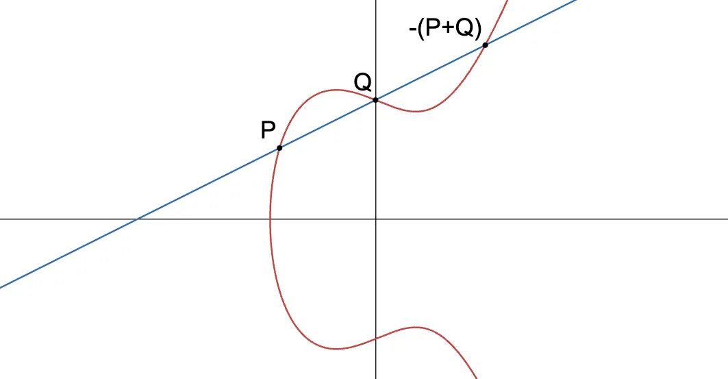
Perhaps more surprisingly, the line also “intersects” $\mathcal{O}$. The reason for this is revealed when looking at projective coordinates:

$$\frac{Y^2}{Z^2} = \frac{X^3}{Z^3} + a\frac{X}{Z} + b$$

We can see that there’s a pole (or singularity, or a point where a function goes to infinity, so to speak) at $Z = 0$, and $Z$ appears three times. It should come as no surprise that the multiplicity of $\mathcal{O}$ is $3$.

All in all, the divisor for a line $\ell$ is:

$$(\ell) = (P) + (Q) + (-(P + Q)) - 3(\mathcal{O})$$

If you think about it, what we have here is a representation of the roots and poles that result from substituting $\ell$ into $E$. We can see that roots have positive multiplicities, while poles have negative multiplicities.

In general, the divisor of a function $f$ is defined as:

$$(f) = \sum_{P \in E(\bar{\mathbb{F}_p})} \textrm{ord}_P(f) . (P)$$

Where $\textrm{ord}_P(f)$ represents the multiplicity of point $P$.

Another cool thing about divisors is that we can add them together. And also, there’s a very useful translation from algebra between functions, to their divisors:

$$(f.g) = (f) + (g)$$ $$(f/g) = (f) - (g)$$

This may not look very inspiring at first. But think about it: just adding or subtracting divisors tells us something about the intersection points of quotients or products of functions with a curve. That’s powerful, because we may not even know the shape of those quotients or products. This will come in handy very soon.

Divisors and Groups

What follows is a bunch of definitions that will take us on a journey exploring the group structure of divisors.

Bet you weren’t expecting that one!

It’s gonna get a little more dicey. Let’s take it slow.

Divisors on a Curve

Of course, an elliptic curve (well, really, any curve) has many divisors. Over the real numbers, it has infinitely many, actually. But over finite fields, the set of divisors of a curve becomes finite.

We denote the set of all divisors of a curve $E$ as $\textrm{Div}(E)$.

We should also specify the algebraic closure of the field as a subindex, but for simplicity, we can ignore it. And also, I just can’t write that with unicode characters!

Because we can add divisors together quite naturally — but we can’t multiply them together — the set of all divisors on a curve forms a group. The rules are simple. Addition works as you’d expect:

$$a(P) + b(P) = [a + b](P)$$

And the identity of the group is the zero divisor: a divisor where every $n_P$ is zero.

Now’s a good time to introduce a couple handy definitions:

• The degree of a divisor is defined as the sum of all its $n_P$ values.

$$\textrm{Deg}(D) = \sum_{E(\bar{\mathbb{F}_p})} n_P$$

• The support of a divisor $D$ is the set of all point that have a non-zero $n_P$:

$$\textrm{supp}(D) = \{P \in E(\bar{\mathbb{F}_p}) \ : \ n_P \neq 0 \}$$

How are we doing so far? Good?

If by this point you’re feeling a bit lost, I recommend re-reading the story up to this point. What follows builds up on all the previous ideas and definitions.

And it’s gonna get crazier. Sorry.

Divisor Subgroups

Some divisors in the overarching group are more interesting than others. And some of those subsets of divisors form proper subgroups. Let’s look at a few of them.

The easiest subset to distinguish is the set of degree-zero divisors, $\textrm{Div}^0(E)$:

$$\textrm{Div}^0(E) = \{ D \in \textrm{Div}(E) \ / \ \textrm{Deg}(D) = 0\}$$

This forms a proper subgroup, because adding together divisors whose degree is zero will result in another divisor of degree zero, landing back on the subgroup.

And just what might be appealing about this subgroup? Well, two things. One is that it contains yet another subgroup of interest.

The other reason will become apparent in just a minute.

Principal Divisors

When $D$ is the divisor of a function $f$ (denoted $(f)$), we call this divisor principal. The set of all principal divisors is denoted $\textrm{Prin}(E)$.

Principal divisors have one defining characteristic: their degree is always zero. This is a profound result, tying back to Bézout’s theorem, which I don’t think is worthwhile to pursue now.

Just believe me on this one. It’s a deep, deep rabbit hole.

This brings up a question, though: is every degree-zero divisor a principal divisor? In other words, given a degree-zero divisor $D$, can we always find a function $f$ such that $D = (f)$?

The answer is no. Again, for reasons we won’t cover. Principal divisors are yet again a subgroup of the degree-zero divisors.

There’s a cool relationship between these groups, though — and this is where the second reason of interest for the zero-degree divisors comes in.

The Picard Group

To establish said relationship, we first need to define divisor equivalence.

Two divisors $D_1$, $D_2$ are equivalent if they can be expressed as $D_1 = D_2 + (f)$ for some function $f4. We usually denote this by$D_1 \sim D_2$.

We can observe a few things:

• When $D4 is the divisor of a function, it’s equivalent to the zero divisor.
• When we choose some non-principal divisor $D’$, we can generate new equivalent divisors by adding other principal ones. Similar to how the modulo operation works.

These ideas naturally lead us to the star of all divisor groups. La crème de la crème — the divisor class group (also called Picard group). It’s defined as the quotient group:

$$\textrm{Pic}^0(E) = \textrm{Div}^0(E) \ / \ \textrm{Prin}(E)$$

Said differently, is the set of all degree-zero divisors modulo the principal divisors. The idea is that elements in $\textrm{Pic}^0(E)$ are irreducible in a sense, and can generate a whole set of equivalent elements when we add function divisors to it — an equivalence class.

Irreducible. Hm. I mean, we know how to calculate modulo when dealing with finite fields. But... How do we calculate the modulo of a divisor?

Divisor Reduction

Calculating the “modulo” of a divisor is more involved than standard integer modulo calculation. But it can be done.

Before we see the process in action, we need a couple more definitions:

• A divisor is effecive if every $n_P$ is greater than zero. In $\textrm{Div}^0(E)$, there’s a single effective divisor: the zero divisor!
• Because of that, we can define the effective part of a divisor, defined as:

$$\epsilon(D) = \sum_{P \ / \ n_P \geq 0} n_P(P)$$

• The size of a divisor is the degree of its effective part.

Equipped with these new concepts, let’s jump straight into how divisor reduction works.

Consider a divisor $D = (P_1) + ... + (P_9) — 9(\mathcal{O})$, of size is $9$. This is clearly an element of $\textrm{Div}^0(E)$ — but we want to find its equivalent element in $\textrm{Pic}^0(E)$.

What we do now is interpolate the $P_i$ points. It should be noted that all these points are on the curve $E$.

For reference, you can check my article on polynomials.

Interpolation will yield this function:

$$\ell_8: y = \sum_{k=0}^8 a_kx^k$$

Now, if we substitute this function into $E$, we’ll obtain a polynomial of degree (at most) $16$, because of the $y^2$ term in $E$. This polynomial will then have $16$ roots.

These roots are the points of intersection between $\ell_8$ and $E$. But notice that the nine $P_i$ points are also points of intersection — they belong to both $\ell_8$ and $E$ as well. This means that through this process, we gain knowledge of a total of seven new points of intersection.

Okay! Let’s use this information to write the divisor of $\ell_8$. We can separate it as:

$$(\ell_8) = \sum_{i=1}^9 (P_i) + \sum_{j=1}^7 (P'_j) - 16(\mathcal{O})$$

And look at what happens after we reorganize that equation a bit:

$$\sum_{i=1}^9 (P_i) - 9(\mathcal{O}) = \sum_{j=1}^7 (P'_j) - 7(\mathcal{O}) - (\ell_8)$$

See what happened? On the left-hand side, we have our original divisor $D$. And on the right, we have a the divisor of a function $(\ell_8)$, and a new divisor whose size is two less than $D$. Let’s call it $D’$.

The difference between $D$ and $D’$ is a function divisor. You know what that means? That $D$ and $D’4 are equivalent!

We can keep repeating this process over and over, using the new divisor’s points for interpolation. Until... When? When do we stop? When do we get an irreducible divisor?

If you try this yourself, you’ll find that you can get to a size-one divisor of the form $(P) - (\mathcal{O})$.

That’s as far as you can go. In short, every point on the curve represent an equivalence class.

This is no coincidence. It’s in fact a consequence of an important theorem, called the Riemann-Roch theorem — one of the most pivotal results in a branch of mathematics called algebraic geometry.

Algebraic geometry is a topic I’d like to tackle in some future article. I don’t think we should go any deeper. Still, a little explanation of what the theorem is about might help.

In a nutshell, every curve has a fundamental property called its genus. It has to do with the number of holes in the surface represented by a curve — which is the surfaces formed by a curve when viewed over the complex numbers. Elliptic curves form sort of a doughnut shape — and thus, have genus $1$.

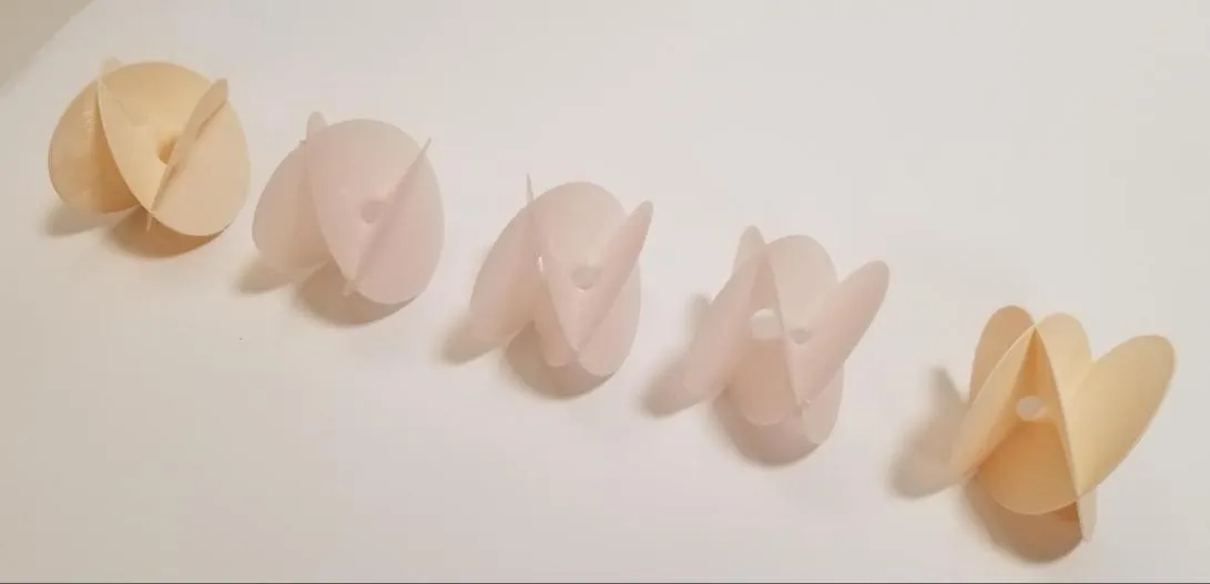
It’s kinda hard to visualize. This post might help.

The Riemann-Roch theorem tells us that any divisor $D$ on an elliptic curve, will be equivalent to another divisor $D’$ whose size is at most $g$, where $g$ is the genus of the curve. In the case of elliptic curves, $g = 1$. Consequently, any divisor of size greater than $1$ can be reduced.

I don’t know about you, but I find these kinds of interactions nothing short of magical. They show how different branches of mathematics are intimately intertwined together, allowing us to look at the same problem through different lenses, and sometimes revealing intricate hidden patterns.

Alright. Perhaps I got too excited there. Sorry.

I may have strayed a little too far our main goal: explaining why point addition works as it does. Time to circle back to that, using our fresh knowledge on divisors.

The Mordell-Weil Group

One of the key results we found is that any divisor of an elliptic curve can be reduced to something of the form $(P) - (\mathcal{O})$. There’s actually a one-to-one correspondence between points in the curve and irreducible divisors of this form.

In other words: there’s an isomorphism between the group of points on our elliptic curve, and the Picard group ($\textrm{Pic}^0(E)$). And the function itself is quite simple: it maps a point $P$ to the divisor class of $(P) - (\mathcal{O})$.

Let that sink in for a moment.

It might not be evident at first. What this means is that our fancy-looking rule for adding points on an elliptic curve (the group law), can be translated into operations in the Picard group.

Here’s how:

• Take two points $P$ and $Q$ on the curve
• Map them to their corresponding divisor classes, which are $(P) - (\mathcal{O})$ and $(Q) - (\mathcal{O})$.
• Add these divisor classes, resulting in $D = (P) + (Q) - 2(\mathcal{O})$.

Now, this is not the standard form in the Picard group—the divisor is reducible. How do we reduce it?

Let’s draw a line through $P$ and $Q$. It intersects the curve at a third point, which we already know is going to be $-(P+Q)$. The divisor of this line $\ell$ is of course:

$$(\ell) = (P) + (Q) + (-(P+Q)) - 3(\mathcal{O})$$

This is a principal divisor, because $\ell$ is a function. Let’s try subtracting it from $D$:

$$D - (\ell) = -(-(P+Q)) + (\mathcal{O})$$

Interesting! This means that $D$ is equivalent to the divisor on the right-hand side. All that remains it to map this to the form $(P) - (\mathcal{O})$. For this, we need to do something akin to negation.

Let’s try using a vertical line going through $-(P + Q)$. It’s a function $v$ with this divisor:

$$(v) = (P+Q) + (-(P+Q)) - 2(\mathcal{O})$$

And this is where the magic happens. Let’s add that to our previous result:

$$D - (\ell) + (v) = (P + Q) - (\mathcal{O})$$

Et voilà! We just need to use our isomorphism (well, its inverse) to map back to elliptic curve points, yielding the familiar $P+Q$.

Let’s shortly analyze what just transpired. All we did was map our original points to divisors, and then add them together. But we added them in the Picard group — and we know we can reduce this result to an equivalent divisor.

The final tie in the knot is the fact that reduction looks exactly like our strange chord-and-tangent rule!

Mind blowing. Simply phenomenal.

Because now, our point addition rule seems to appear naturally when working with the Picard group.

It’s not a crazy invention. It’s just a consequence of learning how to speak the language of divisors, resulting in this addition-and-reduction process, which is the group law for what’s called the Mordell-Weil group.

Pretty neat, huh?

Multiplication, Revisited

To round things up, I want to look at point multiplication from the perspective of the Mordell-Weil group.

Suppose we want to compute $[4]P$, given some point $P$ in the curve. There are two ways we can do this: either add $P$ to itself 4 times, or compute $[2]P$ first, and then double that result.

It’s not immediately clear that both operations give the same result. But now, we can use the Picard group to inspect both approaches. We start with the divisor $(P) - (\mathcal{O})$. Doubling this divisor (class) yields:

$$D = 2(P) - 2(\mathcal{O})$$

Since this divisor has size $2$, we know it’s reducible. Same approach as before — subtract the divisor of the line tangent to $P$, and add the divisor of the vertical line going through the third point of intersection. Working out the math, this simply yields:

$$D - (\ell) + (v) = ([2]P) - (\mathcal{O})$$

It’s at this point that we can take either of the two routes:

• One option is to double $[2]P$. By the same logic, we can find the corresponding divisor, which is $2([2]P) - 2(\mathcal{O})$. Let’s call this $D_1$.
• The other is to add $P$ two more times. This yields $([2]P) + 2(P) - 3(\mathcal{O})$. This result, we’ll call $D_2$.

If we can show that these two divisors are equivalent, then both results will be one and the same. And really, it’s as easy as calculating their difference:

$$D_2 - D_1 = 2(P) - ([2]P) - (\mathcal{O})$$

To easily interpret this result, I’ll perform one of those little magic tricks in math: add and subtract $(-[2]P)$, and then also add and subtract $2(\mathcal{O})$.

It’s the same as adding zero, so it’s perfectly fine.

Let me write the result for you:

$$D_2 - D_1 = 2(P) + (-[2]P) - 3(\mathcal{O}) - (-[2]P) - ([2]P) + 2(\mathcal{O})$$

Aha! It’s becoming clearer, isn’t it? Yes, the difference between $D_2$ and $D_1$ is exactly:

$$D_2 - D_1 = (\ell) - (v)$$

Two principal divisors. Which means, my friends, these divisors are equivalent. Both operations reduce to the same value in the Picard group. How fantastic is that?

Of course, we can show the same thing for any number $n$ — nothing’s special about $4$. The mechanism is exactly the same. It might just take some more work.

And there’s probably a way to show this by induction anyway. I haven’t tried, but it could be a fun exercise!

There you have it! We can now confidently say that the double-and-add rule will result in the same point as repeated point addition.

Summary

If you’ve made it this far, I can only thank you for sticking with me through this algebraic jungle.

The amount of mathematical machinery we can find by taking a peek of what’s behind something as innocent-looking as the chord-and-tangent rule is just mind-bending. And it feels fair to say we’re pretty deep into the wood — but you’d be surprised as how much we’re still scratching the surface.

Don’t panic — we’re well past the point of “superficial understanding”. But there’s much, much more stuff to dig into.

Importantly, we’ve built a solid foundation on divisors. I believe we’ve covered enough for today, at least.

But don’t get too comfortable — we’ll put divisors to good use in the next few article, where we explore pairings. It’s gonna be fun!

Before we get there, there are a few more things I want to say about elliptic curve groups. So that will be our next stop. I’ll see you soon.