Understanding AI: Humble Beginnings

Alright! With the introduction behind us, we should now slowly start making our way into the basic theory of machine learning.

To do so, however, we’re gonna need to be able to more or less speak the mathematical language associated with the constructions we’ll be working with.

Learning from data is of course a mathematical problem, so the math will be unavoidable. Sorry!

So what is it we need to equip ourselves with? Well, almost all of Machine Learning (ML) rests on just three mathematical pillars: linear algebra, probability and statistics, and optimization.

Each of these areas can be very challenging in their own right, and the goal for today is definitely not to go for a deep dive on each of these topics. That would not only be of little help at this point, but also, it’s impossible for me to fit the full depth of these branches of math in a single article!

So here’s the game plan: instead of just throwing concepts at you guys, let’s try to gain some sense of the motivation behind why these areas are important in the context of ML and AI. Then, we'll cover only the essentials so that we can start getting acquainted with the core ideas around them.

And then, we’ll further explore the theory in future articles as we go!

Sounds good? If you’re on board with the terms and conditions, then let’s jump straight into it!

The Machine Learning Pipeline

Every time we're faced with a Machine Learning problem, we'll more or less follow the same basic workflow.

Sure, there will be variations - some very minor, some quite complex -, but there are a few steps that are almost always guaranteed to happen in some shape or form. And this is no coincidence: it has everything to do with the fact that there are some fundamental actions that we need to execute to obtain a model that's actually useful.

Thus, a typical ML workflow looks roughly as follows:

1. Collect some data.
2. Choose a model.
3. Methodically adjust the model so that it matches the data.
4. Evaluate whether the model works well.

One may wonder where exactly each of the three pillars fits into this high-level picture. To answer that, we need to zoom in a little more, and start seeing what happens when we get our hands dirty.

And of course, it all begins with data.

Linear Algebra

As we saw last time, we start with a bunch of observations about some system, like our users and their movie watching habits. However, raw data is rarely structured in a convenient way, and it's up to us to cast these observations into a form that we can actually use.

Our first job then will be to decide how we're going to represent observations, and that's where the first of our three mathematical pillars comes in.

What we'll do is select a set of variables, called features, that we believe describe our observations (remember, this is not trivial), and which we can reasonably measure. And we'll take ordered collections of these features, which we call vectors, to be our basic unit of observation.

So for our intents and purposes, Alice stops being a person and becomes a measurable observation - something like $[28, \text{comedy}, 7.2]$. Vectors are represented as ordered lists of numbers or labels (such as $\text{comedy}$), enclosed in square brackets.

Okay, cool! We got something to work with. Naturally though, these vectors are just static objects. So what do we actually do with them?

A whole lot, actually! Remember, our goal is to take these observations and produce a prediction. To predict something, we're gonna need to perform some operations on these vectors, and the language to operate with vectors is... yeah, you guessed it, linear algebra!

I know this might sound scary - after all, linear algebra is quite a vast subject. The good news is we don't need to be experts to start doing some work. We'll start small, and focus on only one basic operation. But don't let appearances deceive you: it's one of the most powerful tools in all of linear algebra!

And we can worry about other more involved tools later.

A Simple Model

To introduce this operation, we'll ask ourselves the following question: what's the simplest possible thing we could do with a vector to produce a prediction?

Say we want a single number that represents how likely Alice is to enjoy some movie, and suppose we've got three features to work with: her age, genre, and average rating. A reasonable idea is to decide how much each feature should count, and then just add everything up.

If we had to eyeball it, maybe we could say that age probably barely matters, so we make it have a small impact in the decision. Average rating likely matters much more, so it should have more influence in the result. One by one, we assign each feature its own multiplier:

$$\text{prediction} = w_1 x_1 + w_2 x_2 + w_3 x_3$$

Where the $x_i$ are the features, and the $w_i$ are the weights we assign to them respectively.

And that's it! Our first model! It's almost embarrassingly simple, isn't it? Just multiply each feature by a number, sum the results, and read off a prediction.

Models like this, built out of nothing but weighted sums, are called linear models. And believe it or not, they'll be our loyal companions for quite a while.

Also, you may notice I conveniently ignored labels, as we're assuming the $x_i$ values are always numbers. For now, this is a comfortable simplifying assumption, but I promise we'll deal with labels down the road.

Now, here's the neat part. Those weights we added? They are themselves just an ordered collection of numbers - in other words, another vector:

$$\textbf{w} = [w_1, w_2, w_3]$$

So what we just did was take two vectors (our features $\textbf{x}$ and our weights $\textbf{w}$), multiply them term by term, and add up the results into a single number. This operation is so important that it gets its own name: the dot product (or inner product), usually written like this:

$$\textbf{w} \cdot \textbf{x} = w_1 x_1 + w_2 x_2 + w_3 x_3 = \sum_i w_ix_i$$

Also sometimes written as $\langle \textbf{w}, \textbf{x} \rangle$.

So in the end, our entire model boils down to a single dot product. We feed in the features, dot them with the right weights, and out pops a prediction. Not bad for a few multiplications and a sum, right?

That's nice and all... but there's just one little problem.

Or two, really - but let's take it one step at a time!

The first of those problems is that we've assumed that our model spits out a trustworthy output. In our example, that's a number that accurately represents how likely a person is to like a movie. But how can we be so sure?

Remember that back in the previous article, one of the main points about the data we're using is that it has noise. Because people rate movies inconsistently, because measurements drift, and because the same person might answer differently based on their mood.

So even with perfect weights (and that's a big if), our prediction can never be exact. In reality, the best we can hope for is a good guess built on top of imperfect information.

And whenever we have to reason about guesses, uncertainty, and noise, we need to base our analysis on an entirely different branch of mathematics, which happens to be our second pillar.

Probability & Statistics

For better or for worse, real-world data is always messy.

Besides our simple recommendation engine example, it's easy to find sources for this noise: people being inconsistent, sensors drifting, occasional typos sneaking into our spreadsheets, you name it.

So if we ever hope to make sense of it, we can't treat each measurement as some exact truth. Instead, we have to treat our observations as the outcomes of a process that's partly random.

This is a subtle but profound shift in perspective. In essence, we start asking a different question entirely: instead of "what is Alice's rating?", we begin to think in terms of "what ratings is Alice likely to give, and how much do they spread around?"

Luckily for us, there's an entire branch of math built specifically for this kind of reasoning: probability and statistics. Once again, it's a very broad area which we cannot hope to cover in just a couple articles. But we won't need the whole arsenal right away - in fact, a handful of ideas will be enough to get us going.

And rather than just throwing those at you out of the blue, I think it's much better to sort of discover them organically, by means of an example. So for this, we'll use an object I'm sure every single one of us has used at some point: a simple six-sided die.

Whenever we roll one of these, we're sure to get a number from 1 to 6. But we don't know which until it lands. That uncertain quantity (in this case, the result of the roll) is what we call a random variable. It doesn't have a single fixed value; instead, it has a range of possible ones, each with some chance of showing up.

Supposing our die is not loaded, each of the six faces is equally likely to land, so each of the numbers has a 1 in 6 chance of happening. We could also ask "what are the chances of getting an odd number?". So we sum the chances of getting either 1, 3, or 5, and we get 3 in 6. Heck, we could even ask "what are the chances of getting any number?", to which the answer is 6 in 6!

If we say then that the total probability (of rolling any number between 1 and 6) is $1$, then the probability of rolling each single number is $1/6$.

Which is not a choice made on a whim: one of the defining axioms of probability theory is that the probabilities of all possible outcomes always add up to $1$.

Alright, so each particular event has some probability. What happens if we put all these probabilities on a plot? We'll get what's called a distribution - and for one die, it's a perfectly flat one.

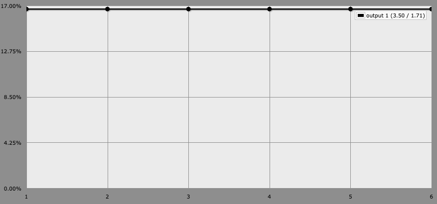
Which might seem boring at first, but it turns out this kind of "flat" distribution (called a uniform distribution) is quite useful for many purposes!

Maybe we can try to shake things up a little. What if instead of one die, we roll two dice, and add the results up? Now the total can be anything from 2 to 12, but what happens to the distribution?

Things get a bit more interesting here, because the outcomes are not equally likely anymore! There's only one way to roll a 2 (1 + 1), but there are six different ways to land on a 7 (1+6, 2+5, 3+4, and so on). So a 7 is six times more likely than a 2.

If we plot this new distribution, we'll soon see it's no longer flat. Now it has a distinct shape, like a pyramid rising in the middle:

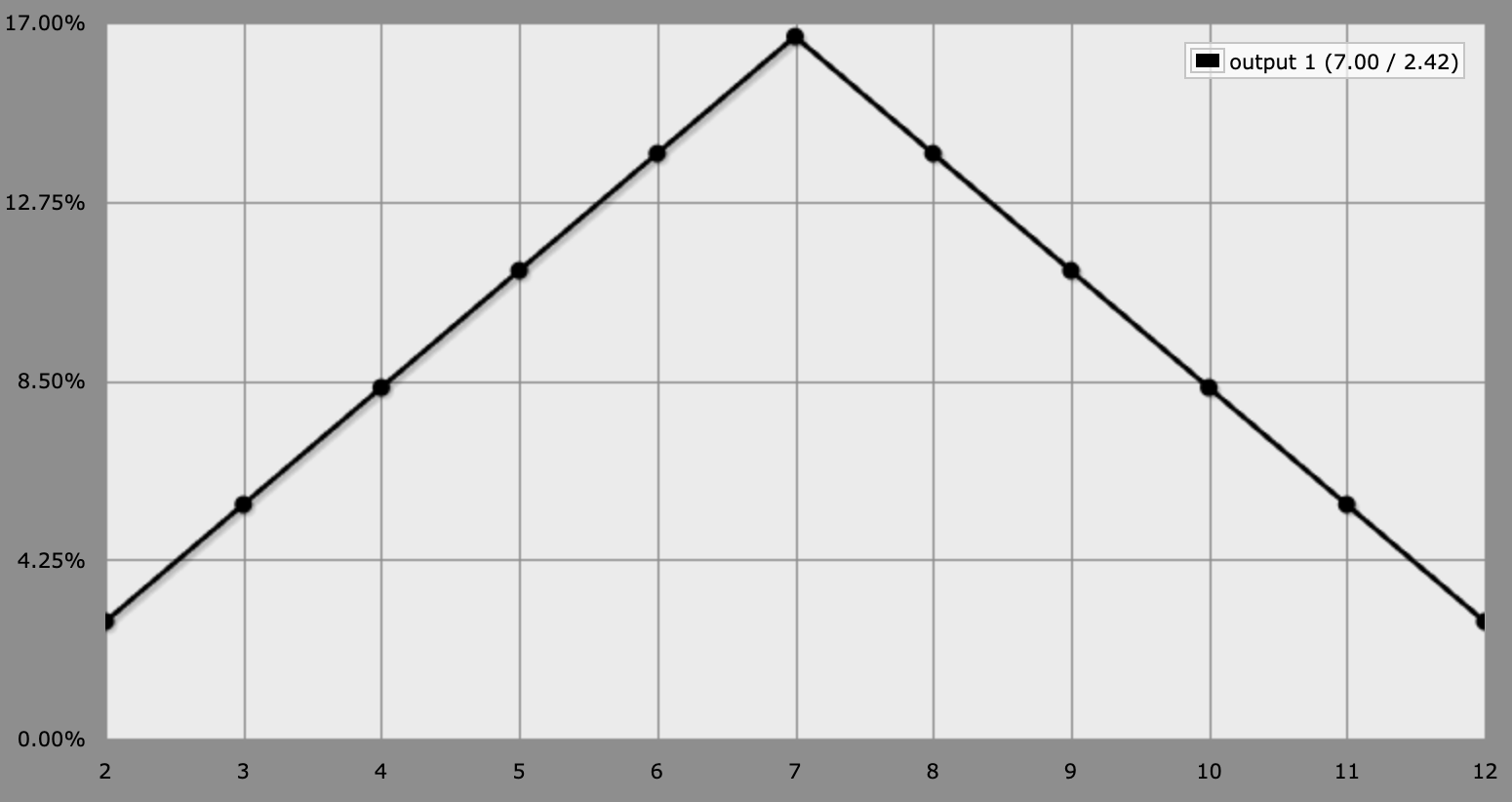
You can see this exact result here.

That's just two dice, and the picture is already quite different. What happens with 3?

Suddenly, we get something that's a little more "curvy" (though still discrete). And if we continue adding more dice, the distribution will become even denser in the center, and values towards the sides will become less and less likely:

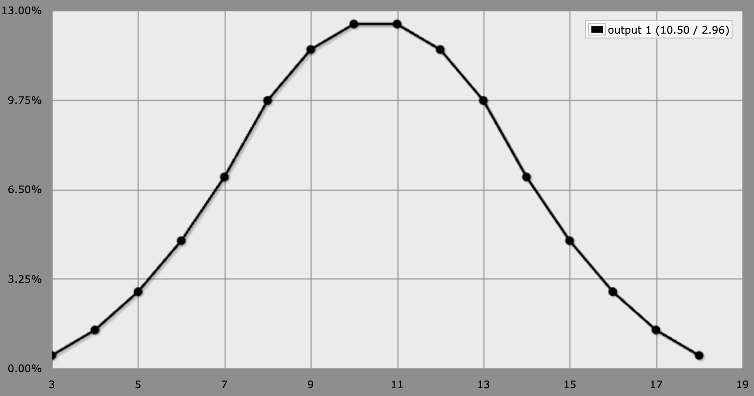
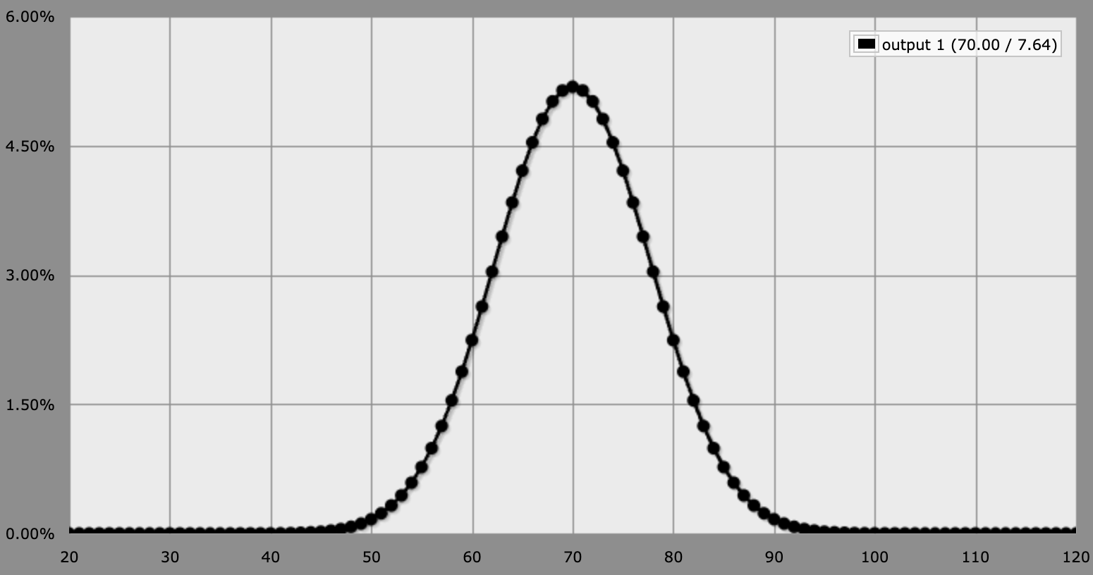
Quite visual, isn't it?

The fact that these distributions mutate in this way as we analyze different random variables is just a testament of what they intend to represent: they tell us not only what can happen, but how likely each outcome is. Some values are typical, others are rare, and we can clearly see this in the spikes and flat zones of a distribution.

Okay, great.. but what does any of this have to do with our movie predictor?

Just about everything! You see, Alice's rating isn't a fixed, set-in-stone number, and it behaves much more like a die roll than one would think. If she watched the same movie on ten different days, she might give it a 7, a 6, an 8... a little distribution of plausible values, with a center (what she'd rate it on average) and a spread (how much her mood pushes it around). And this "noise" we've been talking about all along is precisely how scattered this distribution is!

Which we usually measure with the variance of the distribution. But let's not get ahead of ourselves!

So yeah, by accepting that our data lives in this world of distributions rather than fixed truths, we can begin to think about these problems correctly. Our goal can never be to get exact results, because the very nature of what we're doing forbids it. Instead, we must aim for something different, and much more humble: to be wrong as little as possible.

Which brings us into our third mathematical pillar.

Optimization

Thanks to our previous analysis, we now have a clear goal in mind. But in order to fulfill it, we first need a way to measure how wrong we are!

This is not too much of a problem though (at least conceptually). What we can do is take our model's guesses, compare them against the real data, and boil the mismatch down into a single number - our measure for how badly the model is doing. A number we'd very much like to make as small as possible.

This measure of wrongness is so central to ML that it gets its own name: we call it a loss function, and usually denote it with $\mathcal{L}$.

And mind you, choosing a correct loss function isn't always an easy task. We'll see this in action in due time though!

Adjusting the Loss

Now... remember when I said we had two problems to deal with? Well, it's now time to talk about the second one!

Suppose we have a loss function $\mathcal{L}$ we can use. The other two things we have are some predictor, which we'll call $f$, and a bunch of data points, so pairs of feature vectors ($\textbf{x}$), and an expected prediction $\textbf{y}$ (a rating, in our toy example).

To get a measure for how correct our model is, we just calculate $f(\textbf{x})$ for all our data points (the prediction), and feed both these predictions and the actual measured values $y_i$ into the loss function. But... that's a fixed value, isn't it?

Indeed, we'll get something like $\mathcal{L} = 100$. And then what? A fixed result like that one doesn't really hold much meaning, and it doesn't seem very useful either. So what's the catch? Did we do all this for nothing?

The thing is, we've conveniently swept something under the rug earlier. Remember our simple predictor, using a few weights? Well, we never said where those weights come from!

Yeah! There's no need to blindly guess what the correct weights need to be. Instead, we can do something much smarter: we try to find the values that reduce the loss to a minimum!

When we put it like that, the loss function stops being a static thing, and instead it becomes a function of the parameters of our model (which are just the weights, in this case). And in mathematics, whenever we search for the minimum (or maximum) of a function, what we're doing is optimizing!

An Extra Requirement

Optimization, however, comes coupled with a little bit of extra baggage. You see, finding a minimum is a methodic and systematic endeavor, which relies on calculus.

Please don't run away just yet! I promise it's not as scary as it sounds.

The central idea we'll need is that of the derivative. Oversimplifying a little, a derivative tells us the slope of a function at a given point. This is, if we imagine our function as a sort of multi-dimensional hill, and we stand on a given point on it, the derivative (or the gradient, which is the multi-dimensional cousin of the derivative) tells us in which direction the hill is steepest.

And that's exactly the kind of information we need!

Suppose we have our model with some weights, and we calculate the value of the loss function. When we also calculate the derivative, it gives us a hint of in which direction to nudge our weights, so that we get a smaller loss function value! After doing this enough times, we'll most likely end up very close to a minimum, meaning that we've found a good set of weights!

Optimization in general is a little more complicated than that. We need to ask ourselves things like whether we're close to a local minimum or a global one, and depending on the specific shape of the function, this process might be painfully slow. But again, we'll worry about that later!

This strategy is very much at the heart of machine learning, and it has a name of its own: gradient descent. And we'll see it in action properly in a couple articles, as we churn through our first examples.

Do I Need to Know Calculus?

So, do we need to know how to calculate derivatives in order to do machine learning?

It depends! Much of the time, the optimization machinery will be working quietly under the hood, as it's usually baked into libraries, and because we'll be more interested in what it can achieve rather than grinding through the math ourselves.

But if we want to well and truly understand what's happening (and this will in part be the goal of this series), then yes, we'll need to understand how to calculate derivatives. Rest assured though - I'll be your guide through the entire ordeal, and we'll take the time to churn through the specific calculations.

Summary

So there we have it! Those are the three mathematical pillars that hold up just about everything in Machine Learning (and AI alike).

Sure, we didn't go very deep into any of these areas, but that's very much on purpose. Not only would it be impossible to summarize everything there's to know into a single article, but it would also only confuse us, more than anything.

What I hope stuck with you isn't a bunch of definitions, but rather a feel for why each pillar earns its place:

• Linear algebra gives us the language to represent our data as vectors, and to operate on them.
• Probability and statistics forces us to accept that our data is noisy, and reframes how we think about learning from data.
• And optimization turns that goal into an actual procedure: measuring our "wrongness" with a loss function, and then tweaking our weights (or model parameters) to make it as small as possible.

We've barely scratched the surface (and dodged most of the actual calculations like Neo on Matrix). But fret not - we'll pick these up properly along the way, as we build intuition about the things we'll be doing.

So, where to next?

Well, thus far, everything has been rather abstract. We've got the pieces, but we haven't actually built anything yet!

It's high time we put these three pillars to work, all at once, on a real model. And we'll start with the simplest ones we can find: linear models. If you squint, you'll realize we've already built most of it in this very article!

So it's just a matter of putting the icing on top.

Next time, we'll roll up our sleeves and train our very first models from scratch. See you there!