The ZK Chronicles: Computation Models

Hey! Glad you survived the previous article!

No need to play it tough, I know it was probably a lot. Sorry for that.

Perhaps the most important conclusion from our last encounter was that we could show that verifying general computation efficiently is possible. But then, we also mentioned that we rarely write programs as arithmetic circuits. I mean... To each their own, but what kind of a madman would you have to be to write programs as connected addition and multiplication gates?

Instead, we usually use higher levels of abstraction, in the form of programming languages. We use loops, conditionals, functions. What do we do about those?

What about my Python program, bro?

Jokes aside, the real question at play here is: why circuits? And even though we’ve made some good points for them, like their decomposability, it’s hard to shake the thought that we’d want to prove things about other types of programs.

So today, I want to guide you through the connections between these different computation models. These will reveal some core aspects of verifiable computing in general, and open up a world of possibilities.

I don’t know about you, but this sounds exciting! Let’s dig right in!

Computation

Our journey today begins with a simple question: what does it mean to perform a computation?

At first glance, this might seem like a silly thing to ask. You write code, the computer executes it, you get a result. Where’s the complexity in that?

But if we think about it more carefully, things start getting interesting. For example, writing a program to add two numbers in JavaScript is not the same as writing Assembly instructions to add two numbers. Nor is writing a circuit to add two numbers.

Are these all the same computation? They certainly look different, using a different syntax, different operations, and perhaps most obvious, different levels of abstraction. We go from the simplicity of a circuit gate, to the complex architecture of a CPU, to all the interpreted shenanigans of JavaScript.

Yet intuitively, these examples all do the same thing: they add two numbers!

This matter is at the very core of computation theory: what does it mean for different processes to compute the same thing? And more importantly: are some models of computation fundamentally better or more powerful than others, or are they all equivalent in some sense?

It should come as no surprise that there’s a whole branch of math (and computer science) dedicated to studying these types of questions about computation models.

Computational Complexity Theory

In short, computational complexity theory is the study of what can and cannot be computed efficiently.

One of its core concepts is that of complexity classes: groups of problems with equivalent difficulty, for which we could try to find efficient algorithms.

Thus, we can study models for computation to solve problems in these classes, rather than catering for any particular problems.

These models for computation are really mathematical abstractions that capture the essence of what it means to “compute something”, irrespective of programming languages or hardware.

Here are some of the main models complexity theory studies. Some of them will surely ring a bell:

• Turing Machines: basically the granddaddy of computation models. Imagine an infinite tape containing cells, which contain symbols. The machine points to a single position in the tape at any time, and can move left or right. Depending on the value of the symbol, and based on a simple set of rules, this pointer to the tape can move left or right to other locations, and even write on the tape. Perhaps surprisingly, despite being absurdly simple, Turing machines can compute anything that is computable.
• Random Access Machines (RAMs): a model closer to real computers, with memory addresses you can access directly. This is essentially how your laptop works under the hood.
• Lambda Calculus: a purely mathematical approach where everything is a function. There are only three operations: defining functions, applying functions to arguments, and substituting variables. No loops, no if statements, no changing variables — just pure function composition!

And then, there are the boolean circuits and arithmetic circuits we’ve been talking about for a few articles now!

Despite looking wildly different on the surface, most of these models turn out to be equivalent in a deep and intriguing way.

The Cook-Levin Theorem

Back in 1971, two computer scientists called Stephen Cook and Leonid Levin independently proved something remarkable that has profound implications for our analysis.

In order to understand their theorem, we first need to talk about a special complexity class, called NP.

NP stands for Nondeterministic Polynomial time, and is the class of problems where you can verify a solution quickly (in polynomial time), but finding said solution is considered hard (at least, taking more than polynomial time).

If you squeeze your memory a bit, you’ll remember we already talked about this in the very first article, when we mentioned Sudoku!

With this, we can now jump into the Cook-Levin theorem. We’re not gonna prove it though, because that would take far more than a single article! Plus, the statement alone will give us a lot to process. Here:

Any problem in NP can be reduced to circuit satisfiability in polynomial time

Yeah! Remember our circuit satisfiability (CSAT) problem? Not only does it turn out to be an NP problem, but it’s also equivalent to every other NP problem out there (up to a polynomial time factor).

The way I framed the discussion between circuit satisfiability and circuit evaluation ended up painting a very different picture on the importance and generality of circuit satisfiability... That couldn’t be further from the truth, as we now know!

So in the end, circuit satisfiability has a central theoretical role. Because of the Cook-Levin theorem, we can take any NP problem, and convert it to a CSAT instance. The theorem guarantees this is possible, but of course, the mechanisms may vary.

Once we have our CSAT instance, we can produce an arithmetic circuit. Which allows us to conclude:

Arithmetic circuits are a universal model for bounded computation

Yup! Any computation we care about can be expressed as an arithmetic circuit. This is the main reason we’ve been studying circuits so far, apart from the interesting features they possess: they are mathematically simple, decomposable, possibly structured, and now on top of that, universal.

There’s also another nice consequence to this: we could use CSAT as a pivot point to show that any two NP problems are equivalent.

Click to zoom

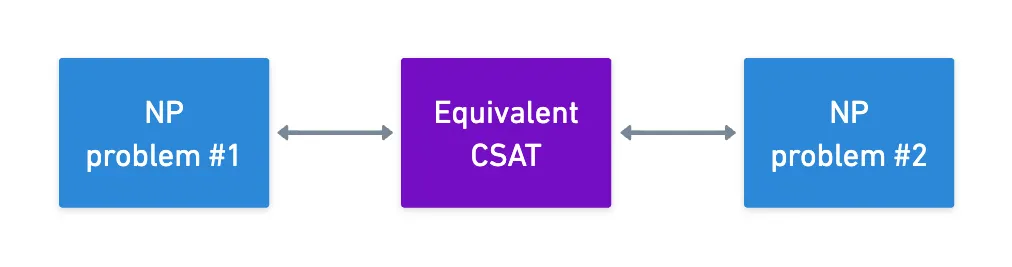
What’s really cool about this is that we could potentially find a very efficient proving system for a particular NP problem, and we could at least in theory convert any other NP problem to that form — of course, with the associated transformation costs (which we usually call a blowup factor).

This hints at a powerful subtlety: with appropriate transformations, we can apply any proving algorithm to any problem!

Whether this is a good strategy or not... That’s another story!

Languages and Decision Problems

Alright! We’ve successfully established that circuits are universal.

While this has immense theoretical value, there’s a subtle shift in perspective we need to make explicit — one that will become crucial as we move deeper into ZK systems.

A Peek into ZK

To motivate this, let’s briefly further our discussion about zero knowledge from the very first article.

It’s still too early for us to formally define what we understand by zero knowledge. That doesn’t mean, however, that we can’t start closing in to the actual definition through slightly more sophisticated concepts.

One thing we didn’t know back then is that we can use circuits to represent computations. Now that we do, we can roughly define what ZK means. It goes like this: a prover will try to convince a verifier that they know some input $w$ to a given circuit so that the output of the circuit is a given value:

$$\varphi(w) = 0$$

The expected output value is usually $0$. And any circuit is easily converted to this format by adding an extra gate that subtracts the expected output.

What makes this zero knowledge is that the verifier can be convinced without ever knowing $w$.

Simple enough, right?

Notice that in the above formulation, the verifier never really cares about the actual value of $w$, just that one such $w$ exists, and this question only has two valid answers: yes and no.

Problems stated in such fashion are called decision problems, and they stand in the direct opposite end of the type of problems where we might actually care about finding a valid solution to a problem.

For example, we want to find an input that satisfies a circuit!

This type of problem is called a search problem, and I guess they might feel more natural for most people. We have a problem, we find a solution that works, boom. Who cares about all the possible solutions?

Well, ZK does: the verifier only needs to know that a valid solution exists, without gaining knowledge of its value!

Plus, the two types of problems are closely related: if you can solve the search problem, you can obviously solve the decision problem (because you’ve found a solution!).

The other direction is a little trickier, but generally speaking, if you can solve the decision problem efficiently, you can often solve the search problem efficiently too. This is done through a technique called self-reducibility.

To this extent, computational complexity theory studies decision problems using a very rigorous mathematical framework, called languages.

Languages

Before you ask: no, this has nothing to do with programming languages like Python or Rust.

A language is just a set of strings that encode yes instances of a problem.

I think this is easier to understand with an example. Let’s consider the following problem: when given some number, we ask “is it prime”?.

Of course, you could go ahead and write an algorithm to determine this. But conceptually, there’s something else we can do. Let’s define the set $\mathcal{L}_p$ as:

$$\mathcal{L}_p = \{2,3,5,7,11,13,17,19,23,...\}$$

Or perhaps more succinctly:

$$\mathcal{L}_p = \{n : n \ \textrm{is prime}\}$$

It should be crystal clear what we meant now: this is exactly the set of all strings (in this case, numbers) for which the answer to our original question is yes. And checking whether a number is prime, provided we know this language in advance, is as simple as checking if the number belongs to $\mathcal{L}_p$.

And I know what you’re thinking: what’s the point?

In our example, how is finding $\mathcal{L}_p$ (which is of course an infinite set) any easier than determining if a single number is prime?

Yeah, it might seem like a pointless formalism, but languages are actually quite powerful. By framing problems in these terms, we can:

• Talk precisely about what it means to solve a problem (finding a value that belongs to $\mathcal{L}$).
• Define complexity classes as sets of languages.
• Reason about reductions between problems.

For instance, our general circuit satisfiability problem can be stated as a language:

$$\mathcal{L}_{\textrm{CSAT}} = \{\phi : \exists x \ \textrm{s.t.} \ \phi(x) = 1\}$$

This is the set of all circuits that have at least one satisfying input. The decision problem then asks whether a particular circuit $\phi(X)$ is satisfiable, which is equivalent to asking whether it belongs to the language!

Alternatively, we could define another language for a specific circuit, as the set of all its satisfying inputs. In that case, the solution to #SAT (the counting problem) simply returns the size of said language!

Witnesses

Now, here’s where things get interesting for ZK.

We mentioned that NP problems are those for which we can verify a solution quickly. And since we’ve already moved into formal theory, perhaps now’s a good time to more precisely define what we mean by verifying.

In the language framework, verification involves three pieces:

• The problem instance ($x$), which represents the problem we’re trying to solve (i.e., a specific Sudoku puzzle, a given circuit).
• The witness ($w$), which is just a piece of evidence that proves $x$ has a solution.
• The verifier ($\mathcal{V}$), which is an algorithm that checks whether $w$ is valid evidence for $x$.

With these pieces, we can formulate the following: a language $\mathcal{L}$ is in NP if there exists a polynomial-time verifier $\mathcal{V}$ and a polynomial-size witness $w$ such that:

$$x \in \mathcal{L} \iff \exists w : \mathcal{V}(x, w) = 1$$

Yeah... What the hell is that?

Relax, I’ve got you. In plain english, what this is saying is that for NP problems, a solution to $x$ can be verified in polynomial time (so, quickly) by the verifier $\mathcal{V}$ thanks to the use of the witness $w$.

But what might this $w$ be? Our two examples so far reveal:

• In Sudoku, $x$ is a partially-filled grid, $w$ is the complete solution to the puzzle, and $\mathcal{V}$ simply checks that all rows, columns, and squares contain all numbers from $1$ through $9$.
• In CSAT, $x$ is the circuit we’re dealing with, $w$ is an input that satisfies the circuit (so, outputs $1$ or $\textrm{TRUE}$), and $\mathcal{V}$ works by evaluating the circuit with input $w$, and checking the obtained output.

Verification is obviously fast in both cases. The witnesses might raise some eyebrows, though: they are valid solutions to the problem!

Wait... Valid solutions? That means the verifier will learn the solution to the problem! Doesn’t that break our definition of zero knowledge?

Instead of going into panic mode, I guess it’s much better for our mental health to ask ourselves this fundamental question: is it possible for the prover to keep $w$ private, but still somehow convince the verifier that $x \in \mathcal{L}$?

As in: “I know an input to this circuit ($w$) that makes the output $\textrm{TRUE}$, but I’m not telling you what it is... And I can still convince you!”.

Of course, this is absolutely possible (we wouldn’t be here otherwise!).

The key point is that we can try to prove that $w$ exists, without revealing it. And this is the quintessential aspect that defines zero knowledge.

Moreover, the witness doesn’t always have to be the complete solution. It just needs to be sufficient evidence. Advanced ZK systems use compressed or cleverly-structured witnesses, which helps make proofs more efficient.

Alas, all this is easier said than done. We’ll start looking at ways to do this in due time, but this new languages framework at least gives us a cleaner way to formulate our goal:

To prove $x$ belongs to the language, while hiding the witness $w$.

In other words: prove that a circuit is satisfiable, without revealing the actual satisfying input!

From Theory to Practice

Alright, we’ve covered a lot of theory. Circuits are universal, languages give us a formal framework, witnesses help with ZK, yeah, yeah... But how does this actually help me prove things? How does this actually work in practice?

Well, after all this theoretical bombardment, here’s a piece of good news: you don’t manually write arithmetic circuits.

That would be insane!

The Cook-Levin theorem we saw earlier allows us to do something quite nice: we can build compilation pipelines that transform any computation into a provable form.

For this, modern ZK systems use a frontend-backend architecture.

In a nutshell, what you do is write your computation in a more natural way, using either:

• Domain-Specific Languages (DSLs) like Circom or Noir, where we write circuit-like code that’s still more human-readable than freakin’ gates.
• General-purpose languages, like Rust or Python.

Frontends process these representations, and transform them into suitable forms that are simply algebraic representations of circuits, such as R1CS, PLONK arithmetization, and AIR.

Don’t worry, we’ll look at what those are later!

Then, backends take these circuit representations and use proving systems (like GKR, or others we’ll explore later) to generate the actual ZK proofs.

Of course, this entire pipeline would not be possible if not for the theoretical results we covered today!

Cook-Levin guarantees that any computation can be reduced to a CSAT problem, which gives us huge versatility. Of course, these transformations have costs, and the different proving systems make different tradeoffs, or may even be tailored for specific situations — so we’ll have to be careful with our selections.

But hey, at least we have some wiggle room!

Summary

That’s enough theory for today!

Our simple initial question led us down an intense theoretical path in computational complexity theory — the study of different models of computation and their relationships.

This revealed important things: models are fundamentally equivalent, and problems can be converted between one inside the same complexity class (up to a polynomial blowup). In particular, the Cook-Levin theorem shows how any NP problem can be reduced to circuit satisfiability, which says something about the universality of circuits.

We also introduced a crucial framework: languages and witnesses. This is a different way to think about problems. It might seem a little strange for now, but it’s a powerful set of tools for formal proofs. We’ll make use of languages later down the road, but for now, just keeping their existence in the back of your mind is enough.

If you’re here after all these shenanigans, congrats! This is probably the single hardest theoretical jump in the series. Sure, we’ll need to talk about other theoretical concepts later, but for me at least, this was the most complicated part to write, or even wrap my head around.

So next time, we’ll start building on all the foundations we’ve covered so far, using some ideas that will probably feel more familiar, and yet, help make verifiable computing and ZK systems actually usable.

Until then!