Cryptography 101: Zero Knowledge Proofs (Part 1)

This is part of a larger series of articles about cryptography. If this is the first article you come across, I strongly recommend starting from the beginning of the series.

It’s finally time for some zero knowledge proofs!

Previously in this series, we outlined what they are. This time around though, we’ll be more thorough in our definition, and look at a more advanced example.

The general idea of a ZKP is to convince someone about the truth of a statement regarding some information, without revealing said information. Said statement could be of different natures. We could want to prove:

• knowledge of a discrete logarithm (the Schnorr protocol)
• a number is in a certain range
• an element is a member of a set

among others. Normally, each of these statements requires a different proof system, which means that specific protocols are required. This is somewhat impractical — and it would be really nice if we could generalize knowledge proofs.

So our plan will be the following: we’ll look at a ZKP technique, called Bulletproofs. We’ll see how they solve a very specific problem, and in the next few articles, evaluate how almost the same thing can be achieved in a more general way.

We’ll just focus on the simple, unoptimized version (it’s complicated enough!). And if this article isn’t enough to satiate your curiousness, either the original paper or this article here might be what you’re looking for.

Let’s start with a soft introduction to the topic, before jumping into the math.

Zero Knowledge Basics

When we talk about proving validity of statements, the broader family of techniques is called proofs of knowledge. In these types of protocols, there are usually two actors involved: a prover, and a verifier.

And there are also two key elements: a statement we want to prove, and a witness, which is a piece of information that allows to efficiently check that the statement is true. Something like this:

Click to zoom

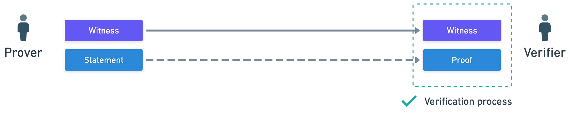
Only that this is not the full story!

If you recall from our brief look at the Schnorr protocol, we saw how there was some back and forth communication between the prover and the verifier. And there’s good reason for this: the verifier provides an unpredictable piece of information to the prover. What this achieves is making it extremely hard to produce false proofs — and very simple to produce valid proofs, so long as the prover is honest. This “wildcard” factor is typically called a challenge.

A Simple Example

To wrap our heads around this idea, here’s a very simple exercise: imagine Alice places a secret sequence of poker cards face down on a table. Bob, who is sitting across the table, wants to check that Alice knows said secret sequence. What can he do about it?

Well, he could ask “tell me what card is in the fourth position”. If Alice indeed knows the sequence, she can confidently answer “7 of spades”, and Bob could simply look at the face down card and check that it matches. Bob has provided a challenge by selecting a card, and it’s only through honest knowledge of the sequence that Alice can provide correct information. Otherwise, she’d have to guess — and it’s unlikely that she’ll say the correct card.

Granted, this is not zero knowledge, because parts of the sequence are revealed!

Adding this challenge into the mix, we get a more complete picture:

Click to zoom

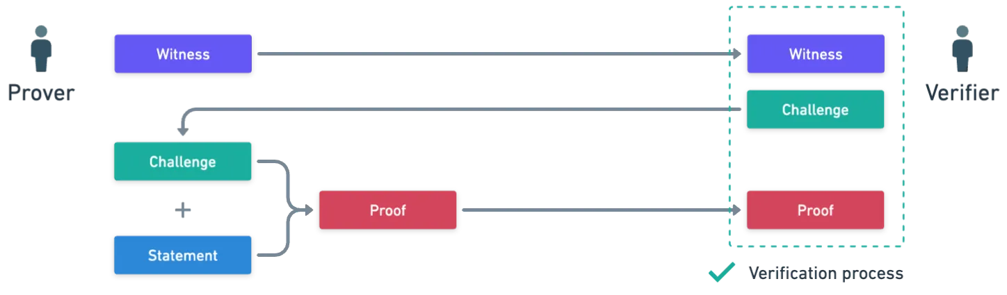
The idea is that the prover makes a commitment to their information, before knowing the verifier’s input (in our example, Alice commits by placing the cards face down)— and this sort of prevents them from cheating.

Formally, the structure we just described is typical of Sigma protocols. You may also see the term Public Coin verifier, which just means that the random choice of the verifier is made public. You know, just to avoid confusions!

To finish our brief introduction, here are the two key properties that proofs of knowledge should suffice:

• Completeness: An honest prover with an honest statement can convince a verifier about the validity of the statement.
• Soundness: A prover with a false statement should not be able to convince a verifier that the statement is true. Or really, there should be very low probability of this happening.

Now, if we add the condition that the proof reveals nothing about the statement, then we have ourselves a zero knowledge proof. We won’t go into formally defining what “revealing nothing” means, but there are some resources that explain the idea if you want to dig deeper.

With this, the intro is over. Turbulence ahead, hang tight.

Range Proofs

As previously mentioned, a crucial element we need to decide upon is what we want to prove. For example, in the case of the Schnorr protocol, we want to prove knowledge of the discrete logarithm of a value.

Another statement we could wish to prove is that some value lies in a range. This may be useful in systems with private balances, where it’s important to prove that after making a transaction, the remaining balance is nonnegative (positive, or zero). In that case, we only need to prove that said value lies in a range:

$$b \in [0, 2^{n-1} - 1]$$

And this is where techniques like Bulletproofs come into play. Now… How on Earth do we go about proving this?

Switching Perspectives

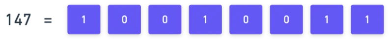
Think of a number $v$ represented by a byte (8 bits). Then, this number can only be in the range of $0$ to $255$ ($2^8 - 1$). So, if we can prove the statement:

There’s a valid 8-bit representation of $v$

Then we have constructed a knowledge proof that $v$ lies between $0$ and $255$. And that’s all we’ll be doing, at its core.

Click to zoom

However, we must turn this idea into a set of mathematical constraints that represent our statement.

To get us started, let’s denote the bits of $v$ by the values $a_{l,0}$, $a_{l,1}$, $a_{l,2}$, and so on — with $a_{l,0}$ being the least significant bit. This means that the following equality holds:

$$a_{l,0}2^0 + a_{l,1}2^1 + a_{l,2}2^2 + ... a_{l,n-1}2^{n-1} = v$$

In order to avoid long and cumbersome expressions, let’s introduce some new notation. Think of our number $v$ represented as a binary vector, each component being a bit:

$$\vec{a_l} = (a_{l,0}, a_{l,1}, a_{l,2}, ..., a_{l,n-1}) \in {\mathbb{Z}_q}^n$$

And also, let's define this:

$$\vec{W}^n = (W^0, W^1, W^2, ..., W^{n-1}) \in {\mathbb{Z}_q}^n$$

We can plug in any value for $W$ — and in particular, plugging in either $0$ or $1$, results in a vector of zeros or ones, respectively.

Now, we can see that the equation from before can be written as an inner product:

$$\langle \vec{a_l}, \vec{2}^n \rangle = a_{l,0}2^0 + a_{l,1}2^1 + a_{l,2}2^2 + ... a_{l,n-1}2^{n-1} = v$$

Ah, the flashbacks from linear algebra

This notation is fairly compact, so we’ll be using similar expressions throughout this article.

If this equation holds, it means that $a_l$ correctly represents $v$, and in consequence, that $v$ is in the expected range. Except, again, that’s not the full story.

We’re missing one tiny detail: the values in $a_l$ might not be zeros and ones! The possible values for each digit or vector component can really range from $0$ to $q$, depending on which finite field we’re using. In other words: each component can be any element in the integers modulo $q$. And the equality might still hold.

So we’ll require an extra condition. For this, we define:

$$\vec{a_r} = \vec{a_l} - \vec{1}^n$$

All we’re doing there, is subtracting $1$ from each element in our vector. Meaning that:

• If some component $a_{l,i}$ has value $1$, then $a_{r,i}$ will have value $0$
• If $a_{l,i}$ has value $0$, then $a_{r,i}$ will wrap around (kind of an underflow, if you will) to $q - 1$.
• Otherwise, neither $a_{l,i}$ nor $a_{r,i}$ will have value $0$.

This is important, because if $a_l$ really is a binary number, something like this should happen:

Click to zoom

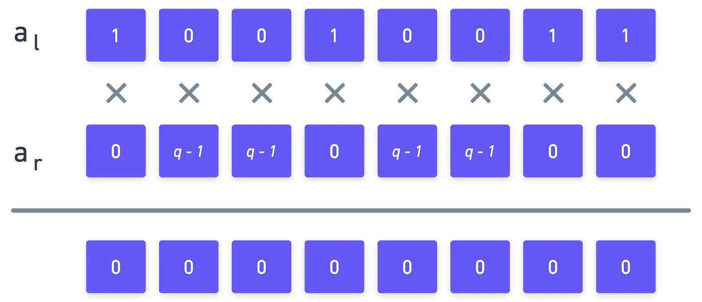
Would you look at that! As long as our binary representation is correct, then the inner product of $a_l$ and $a_r$ will yield $0$!

$$\langle \vec{a_l}, \vec{a_r} \rangle = 0$$

Summarizing, we have a grand total of two conditions that conform our statement (remember, the statement is what want to prove).

$$\left \{ \begin{matrix} \langle \vec{a_l}, \vec{2}^n \rangle = v \\ \\ \langle \vec{a_l}, \vec{a_r} \rangle = 0 \end{matrix}\right.$$

The Protocol

Our system is set. If we know the values of $v$ and $a_l$, then checking that the binary representation is correct is pretty straightforward — we just check that the system holds.

However, since we’re going the zero knowledge route, then the verifier will not know these values. So in order to convince them, the prover will have to do some wizardry — nothing surprising, at this point in the series.

The Commitments

Everything starts with commitments. Remember that commitments can only be opened with valid values — so they bind the prover to the statement they want to prove.

Let’s start by committing to the value $v$. For this, a Pedersen commitment is used. We’ll use a multiplicative group $\mathbb{G}$ of prime order $q$ (see the article about isomorphisms if you need a refresher, or check the previous article), with generators $g$, $h$.

The commitment looks like this:

$$V = g^vh^{\gamma}$$

Secondly, we want to commit to $a_l$ and $a_r$, which are also part of our system. Since these are vectors, we’ll need a slightly more complex commitment. We’ll use generators $g_k$, and $h_k$, with $k$ ranging from $0$ to $n$. Here, the amount of bits in our range will be $n + 1$. And here’s the commitment (drum roll please):

$$A = h^{\alpha}\prod_{i=0}^n {g_i}^{a_{l,i}}{h_i}^{a_{r,i}} = h^{\alpha}{\vec{g}}^{\vec{a_l}}{\vec{h}}^{\vec{a_r}}$$

Woah woah, that’s a lot of symbols right there!. Let’s stop and examine the expression.

The big $\Pi$ symbol is a product, which is like a summation, but instead of adding terms, we multiply them.

In order to make the expression less daunting, we use vector notation. With it, we save ourselves the time of writing the product symbol, but in reality, both expressions represent the same thing.

What’s interesting about Pedersen commitments is that we can combine many values into a single commitment, with just one blinding factor. Nice!

We’ll also require blinding factors for the components of $a_l$ and $a_r$ — these will be two randomly-sampled vectors $s_l$ and $s_r$, to which we commit with:

$$A = h^{\rho}\prod_{i=0}^n {g_i}^{s_{l,i}}{h_i}^{s_{r,i}} = h^{\rho}{\vec{g}}^{\vec{s_l}}{\vec{h}}^{\vec{s_r}}$$

These commitments are sent to the verifier, so that the prover is bound to v, and its binary representation.

The Challenge

Now that the verifier has some commitments, they can proceed to make a challenge. For this, they will pick two random numbers $y$ and $z$, and send them to the prover.

What the prover does now is quite convoluted and confusing, to be honest. And this is part of the point I want to make in this article: maybe trying to craft a more general framework for zero knowledge proofs could be an interesting idea.

The prover will compute three expressions, that really represent a bunch of polynomials ($2n + 1$ in total, to be precise). We’ll try to understand in just a moment — for now, let’s just power through the definitions. These polynomials are:

$$l(X) = (\vec{a_l} - z \cdot \vec{1}^n) + \vec{s_l} \cdot X \in {\mathbb{Z}_q}^n$$ $$r(X) = \vec{y}^n \circ (\vec{a_r} + z \cdot \vec{1}^n + \vec{s_r}) + z^2 \cdot \vec{2}^n \in {\mathbb{Z}_q}^n$$ $$t(X) = \langle l(X), r(X) \rangle = t_0 + t_1X + t_2X^2 \in {\mathbb{Z}_q}$$

I know this is how I felt the first time I saw this:

Lots to unpack here. First, a couple clarifications on notation:

• The dot product ($\circ$) will be interpreted as component-wise multiplication. This is if we write $a \circ b$, then the result will be a vector of the form $(a_0b_0, a_1b_1, a_2b_2, ...)$. This is used in the $r(X)$ expression.
• The scalar product ($\cdot$) is used to multiply every component of a vector by a scalar (an integer, in our case). So for instance, $z \circ a$ (where $z$ is a scalar) will yield a vector of the form $(za_0, za_1, za_2, ...)$.

In particular, let’s focus on the independent term from the very last polynomial, $t_0$. It can be calculated through this expression:

$$t_0 = z^2.v + \delta(y,z)$$ $$\delta(y,z) = (z - z^2).\langle \vec{1}^n, \vec{y}^n \rangle - z^3.\langle \vec{1}^n, \vec{2}^n \rangle$$

Notice that $\delta$ is a quantity that the verifier can easily calculate, which will come in handy in a minute.

Importantly, this term contains the value $v$, which is central to our original statement. In a way, proving knowledge of a “correct” $t_0$ is tied to proving knowledge of $v$. And this is exactly what’s coming next: providing a correct evaluation of the polynomials.

So, the verifier commits to the remaining coefficients of $t(X)$, $t_1$ and $t_2$ — sampling some random blinding factors $\tau_1$ and $\tau_2$, and calculating:

$$T_1 = g^{\tau_1}h^{t_1} \in \mathbb{G}$$ $$T_2 = g^{\tau_2}h^{t_2} \in \mathbb{G}$$

And these are sent to the verifier. But we’re not done yet…

The Second Challenge

For this to work, we’ll require yet another challenge. If you think about it, this makes sense because of how we’ve framed the protocol so far: we have a bunch of polynomials, so now we need to evaluate them.

And thus, the verifier samples a new challenge $x$, and sends it to the verifier. With it, the verifier proceeds to calculate:

$$\vec{l} = l(x), \ \vec{r} = r(x), \ \hat{t} = \langle \vec{l}, \vec{r} \rangle$$

Two more gadgets are required for the proof to work. The verifier needs to calculate:

$$\mu = \alpha + \rho x$$ $$\tau_x = \tau_2 x^2 + \tau_1 x + z^2 \gamma$$

Don’t worry too much about these — they are just needed for the math to work out. They act as composite blinding factors, in fact.

Finally, all of these values (the vectors $\vec{l}$ and $\vec{r}$, $\hat{t}$, and the blinding factors) are sent to the verifier, who finally proceeds to the verification step. Hooray!

Verification

At this point, the verifier has received several values from the prover, namely:

$$V, A, S, T_1, T_2, \mu, \tau_x, \vec{l}, \vec{r}, \hat{t}$$

As previously mentioned, what the verifier wants to check is that the polynomial evaluations are correct. And in turn, this should convince the verifier that $v$ is in the specified range. The connection between these two statements is not evident, though — so I’ll try to give some context as we go.

Linking the Polynomials

The first equality the verifier checks is this one:

$$g^{\hat{t}}h^{\tau_x} \stackrel{?}{=} V^{z^2}g^{\delta(y,z)}{T_1}^x{T_2}^{x^2}$$

If you’re interested, this makes sense because:

$$V^{z^2}g^{\delta(y,z)}{T_1}^x{T_2}^{x^2} = (h^{\gamma}g^v)^{z^2}g^{\delta(y,z)}(g^{t_1}h^{\tau_1})^x(g^{t_2}h^{\tau_2})^{x^2}$$ $$g^{vz^2 + t_1x + t_2x^2 + \delta(y,z)}h^{\tau_2x^2 + \tau_1x + z^2 \gamma} = g^{\hat{t}}h^{\tau_x}$$

What does this all mean? If you pay close attention, you’ll see that on one side of the equality, we have the evaluation $t(X)$, and on the other side, the value $v$ (present in the commitment $V$). So what this equality effectively checks is that the value $t(x)$ is tied to the original value $v$. So, knowledge of $t(x)$ also means knowledge of $v$. This is what the verifier should be convinced about by this equality! In summary:

This check convinces the verifier that $v$ is correct so long as $t(x)$ is also correct

For the next check, we’ll need to define this new vector:

$$h'_i = h_i^{y^{-i+1}} \rightarrow \vec{h'} = (h_1, h_2^{y^-1}, h_3^{y^-2}, ...)$$

As convoluted as this may look, this actually makes the upcoming check work like a charm. The verifier first computes:

$$P = AS^x(\vec{g})^{-z}(\vec{h'})^{z\vec{y}^n + z^2\vec{2}^n} \in \mathbb{G}$$

And then evaluates:

$$P \stackrel{?}{=} h^{\mu}(\vec{g})^{\vec{l}}(\vec{h'})^{\vec{r}}$$

This time I won’t provide proof that the expressions should match — I think it’s a nice exercise in case you’re interested and don’t want to take my word for it!

Whether if you choose to believe me or check for yourself, here’s what’s happening here: $P$ contains the values for all the $a_l$ and $a_r$ values, while on the other side of the equality, we have the evaluations of $l(X)$ and $r(X)$. Because the prover received a challenge from the verifier ($x$), it’s infeasible that $P$ will suffice the equality if the polynomials are incorrectly evaluated. All in all, this is what happens:

This check convinces the verifier that the bit representation of $v$ (the $a$ vectors) are correct so long as $l(x)$ and $r(x)$ are correct

So, finally, we need to check that the evaluations of the polynomials match. And this is very easy to check:

$$\hat{t} \stackrel{?}{=} \langle \vec{l}, \vec{r} \rangle$$

This check ensures that $\hat{t}(x)$ matches the expected value. While it’s simple to choose values of $t(x)$, $l(x)$, and $r(x)$ that conform to this expression, it’s extremely unlikely that they would also suffice the previous two checks. So, in conjunction with them, what this does is:

This check convinces a verifier that the polynomial evaluations are correct

Et voilà! That’s the complete proof. Piece o’ cake, right?

I’ll say this again, since reaffirmation at this stage might be important: this is very convoluted and certainly not simple. But hey, it works!

Summary

I know this was not a light reading — probably quite the opposite. There aren’t many ways to circumvent the complexity of the protocol though, it is what it is! But in the end, we’re able to fulfill our purpose, and we have ourselves a way to prove that a number lies in a given range.

Zooming out a bit, what we can see is that our statement was fairly simple to pose. Three simple equations, and we’re done. Still, we needed some elaborate cryptographic gymnastics to prove it.

And this is completely fine, but it also triggers a certain itch: can we be more general? Is there a more general framework to prove statements?

Indeed, there is. Don’t get me wrong — Bulletproofs and other kinds of tailor-made ZKPs are very cool, useful, and perhaps more performant than a generalized implementation. But if every statement requires specific research and complex implementations, then it may become a bottleneck for new applications.

It is in this spirit that we’ll move on in the series — by exploring a certain framework for more general proofs: SNARKs. But we’ll need to lay some groundwork first — and that will be the topic for the next article!