The ZK Chronicles: Sigma Protocols

As we wrapped things up with the introduction of our very first commitment schemes, we had to point out that even when they hold a lot of potential, they are not proving systems. Although, it sure feels like they are closely related.

We’ll soon discover that their arithmetic properties are the key to developing a new set of proving mechanisms, crafted once again through clever interactions between a prover and a verifier.

The notion of interactive proofs should already feel familiar. We even mentioned something back in our very first encounter!

And so, after a good number of articles spent on setup, we’ll once again turn our attention towards building proving systems. In the process, we’ll uncover some new central concepts that will inch us much closer to the zero knowledge we’re seeking.

This is gonna be a long one. Sit tight, grab a coffee, and let’s dig in!

Sigma Protocols

Rather than a single protocol, today we’ll be looking at a family of protocols, known as Sigma Protocols.

Or Σ-protocols for short!

Conceptually, they are pretty simple, as they are defined by three main phases:

• Commitment: a prover sends an initial message.
• Challenge: the verifier sends a random challenge, which must be unpredictable by the prover.
• Response: The prover responds to the challenge in such a way they are able to prove something about a statement.

The commit-challenge-response relates closely to the etymology of the name “sigma”. Although, I’ve heard at least two versions of the story.

One is that the back-and-forth pattern resembles the greek letter sigma (Σ). Which it does! Plain and simple.

The other, slightly more convoluted, is that the “sig” part comes from the zig-zag-type motion of the messages, and that “ma” comes from Merlin-Arthur, a common convention to designate the prover (Merlin) and the verifier (Arthur).

I’ll let you decide which story you like better!

This pattern should sound very familiar: it’s the same type of interaction we used when defining the sum-check protocol, and the more complex GKR protocol.

Those were pretty interesting in their own right, and of course, in the right context. Much in the same fashion, Sigma protocols have their area of specialization: they are used to prove knowledge of secret values.

Which has a nice zero-knowledge ring to it, doesn’t it?

And we’ll see this in action right away with the most famous example.

Schnorr Protocol

Our initial goal will be as simple as it can be: we’ll try to prove knowledge of a single secret integer $x$.

Nothing more, nothing less! We can worry about the why later.

So, how could we go about this? We already have a sizable set of basic tooling, so maybe we can start by examining what we have!

Recalling our brief passage through groups, we know a simple way to keep a value hidden is by burying it under a discrete logarithm. In other words, when we calculate:

$$y = g^x$$

We know that it’s infeasible to recover $x$ from $y$ (remember, this is notation for applying the group operation $x$ times on $g$).

So, this is the idea: if we can somehow convince a verifier that we know the discrete logarithm of the group element $y$, then we would have proven knowledge of $x$!

This is exactly the concept behind the Schnorr protocol. And to not dangle too long on introductions, here’s how it goes:

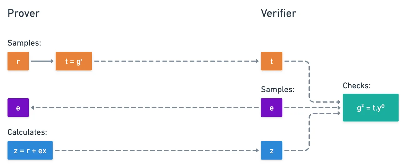
• First, both parties (the prover and the verifier) agree on a group $\mathbb{G}$ of size $n$, and a generator $g$. The value $y$ can actually be made public.
• Then, on the first round, the prover commits to some randomness $r$, by calculating and sending:

$$t = g^r$$

• Upon receiving this value, the verifier samples a random challenge $e$, and sends it back to the prover.

$$e \overset{\$}{\leftarrow} \mathbb{Z}_n$$

• The prover then computes $z$, and sends it to the verifier:

$$z = r + e \cdot x \ (\textrm{mod} \ n)$$

• And finally, the verifier performs this little check here:

$$g^z \overset{?}{=} ty^e$$

Notice how similar this looks to a Pedersen commitment!

If the check passes, then the verifier accepts the proof. Visually:

Click to zoom

Easy, right?

I want to provide an intuitive example of how this plays out in practice. Imagine you, the verifier, are colorblind. In front of you, you have two balls. A prover claims the balls have different colors, but you just can’t see it!

So, you agree to play this game: you first choose a ball, and point it so that the prover can see. Then, the prover turns around, and you get the choice of switching the position of the balls, or keeping them in place. That’s your challenge.

Finally, the prover turns around, and points at the ball you had originally chosen. What’s more, you can keep playing this game, and if the prover guesses right every time, then it’s highly likely that they can see the different colors!

We first want to show that this protocol is complete, or that it works when a verifier is honest. It’s pretty straightforward to show this:

$$g^{z \ \textrm{mod} \ n} = g^{r + x \cdot e \ \textrm{mod} \ n} = g^{r + xe} = g^r(g^x)^e = t \cdot y^e$$

The $\bmod n$ can be safely ignored because, since we’re dealing with cyclic groups of size $n$, we’re guaranteed to obtain the identity every $n$ steps.

To make this more explicit, suppose $z \bmod n = h$. Then, we know that $z = h + k \cdot n$, for some integer $k$. Substituting, we get: $g^z = g^h \cdot g^{kn} = g^h$. This is, we can ignore the modulo operation altogether!

Great! The two values will match, so the algorithm is complete. In fact, it’s perfectly complete: the verifier will always accept a valid transcript $(t, e, z)$.

Next, we need to look at soundness.

Soundness

As we already know, soundness requires us to demonstrate that a cheating prover cannot easily trick a verifier.

Here’s where things get interesting, because there are two flavors of soundness arguments for this protocol. We have the more standard demonstration, and then an even stronger condition that has some cool implications.

Let’s start with the direct approach: how hard would it be for a cheating prover to convince a verifier that they know $x$, without actually knowing it? To answer this, we note that to pass verification, they need to find a pair of values value $(t, z)$ such that verification passes.

First, let’s consider the scenario where the prover knows the challenge $c$ in advance. In this situation, cheating would actually be quite easy: you just pick any $z$, and compute $t$ as:

$$t = g^z y^{-e}$$

Again, remember that this exponential notation represents the group operation. That second term $y^{-e}$ is the inverse of $y^e$ in the corresponding group. That means, for example, that for an elliptic curve group, those points are symmetric with respect to the x-axis!

But because $e$ is sent after committing to the randomness $r$, they have only one of two options: to guess $c$ beforehand, or to guess $x$ once they know $e$.

Both these numbers can be just about any of the possible values in $\mathbb{Z}_n$, and thanks to the discrete logarithm problem, the cheating prover has no better option than guessing. If $n$ is large, the chances of guessing either $e$ or $x$ correctly get absurdly small ($\approx 1/n$), and so, the chances of cheating are effectively negligible!

That’s enough to satisfy soundness. But, we still have a second flavor of soundness to explore!

Special Soundness

One of the things we mentioned before actually has a nice consequence. We know that a cheating prover has little chance of guessing the choice of $e$ from the verifier, right? If guessing a single $e$ value is hard, guessing two independent selections of $e$ (say, $e$ and $e'$) is much, much less likely!

So, suppose we run this Schnorr protocol two times for the same randomness, producing two accepting transcripts $(t, e, z)$ and $(t, e', z')$. Our intuition then tells us that because the prover correctly responded to both challenges, they must know x — because it’s extremely unlikely that they correctly predicted both $e$ and $e'$.

We can actually prove this: if we can extract (or recover) $x$ from the two transcripts, it means $x$ was known by the prover!

Here’s the strategy: since there are two accepting transcripts, we have that:

$$g^z = ty^e, \ g^{z'} = ty^{e'}$$

Let’s divide the first equation by the second. This translates into exponent subtraction, which we know how to work with:

$$g^{z {-} z'} = ty^et^{-1}y^{-e'} = y^{e {-} e'} = (g^x)^{e {-} e'} = g^{x(e {-} e')}$$

Look at that! The first and last members of this equation have the same generator, which means that the exponent must be equal!

Or at least, congruent modulo $n$!

All that remains is to solve for $x$:

$$x = (z {-} z')(e {-} e')^{-1} \ (\textrm{mod} \ n)$$

And boom! We’ve successfully extracted the secret!

The property of being able to extract the witness from two accepting transcripts with the same commitment but different challenges has a name: it’s called special soundness.

It’s a much stronger guarantee than basic soundness, since it tells us that if a prover can successfully answer multiple different challenges for the same commitment, they must actually know the witness. There’s just no way around it!

One small detail for the purists out there: we require the extraction algorithm to run in polynomial time. This ensures the extractor is not just theoretical, but efficient.

Is This Zero-Knowledge?

Ah, the million dollar question!

Yeah, the protocol is complete and sound. But this new special soundness thingy might lead us to think that some information is leaking! What is it then?

It’s clear that the prover’s response $z$ involves the secret $x$. But does it reveal anything about it?

Well, if the verifier had knowledge of the randomness $r$, they could simply calculate:

$$x = (z {-} r)e^{-1} \ \textrm{mod}  n$$

However, because the randomness is unknown to the verifier, and we only use it through clever arithmetic equivalences, the verifier cannot do this! The value $r$ acts as a blinding factor, and the verifier learns nothing about $x$ from $z$.

That’s the intuition, at least — and it should be enough for us to say that the Schnorr protocol is zero-knowledge. We’ll explore the formalisms later, but this does feel like a nice approximation!

Languages Revisited

Lastly, while absolutely needed, completeness and soundness are but the bare minimum set of requirements for verifiable computing techniques to work: they mean that a protocol works for honest provers, and dishonest ones will have a hard time trying to cheat.

We can even throw zero knowledge in there for what it’s worth!

And here, it’s a good time to pause to ask the complementary question: what does an honest prover actually have that a cheating one doesn’t?

The answer is quite obvious, at least in this case: they know $x$. How do we make that more precise, though?

Back when we talked about computation models, we introduced the idea of a language: a set of statements for which a valid witness exists. We didn’t dwell on it too long then, but Schnorr gives us the perfect excuse to work out a concrete example.

So, what’s the language here? It’s just the set of all group elements $y$ for which a discrete logarithm exists:

$$\mathcal{L} = \{y \in \mathbb{G} \ \vert \ \exists x \in \mathbb{Z}_n : g^x = y \}$$

In this case, the witness is simply $x$ itself: the secret integer we’re trying to prove knowledge of, without revealing it.

It might seem that this is just a cosmetic reframing, but it’s actually much more powerful than that. We’re transforming the notion of knowing the discrete logarithm $x$ of some value $y$, into a statement about membership on a set. That is, the prover will be convincing the verifier that $y$ belongs in the language of the elements that have a discrete logarithm (in relation to $g$), and the witness is sort of the certificate that backs up that claim.

Of course, the whole point of this is that the verifier never sees such certificate, but becomes convinced that it exists!

This in turn makes special soundness feel a lot less like a gimmick, and a lot more like a formal guarantee: if a prover can answer two independent challenges for the same commitment, we can extract their witness. And extractability is exactly what we mean when we say a prover knows something, rather than just getting lucky.

We’ll come back to these ideas and make them even more precise later in the series when we look at yet another closely-related concept, called knowledge soundness. It’s a bit of a more general version of special soundness, because it allows unlimited interactions between prover and verifier, but the idea is the same: we’re eventually able to extract the witness, which means the prover must know it.

For now, it’s good to keep this framing in mind — languages and witnesses will keep showing up when we want to formalize things, and they are there even if we don’t talk about them explicitly!

With that, we have quite an extensive covering of the Schnorr protocol.

That’s quite a lot to say about such an innocent-looking procedure!

At this point, one question may be popping in your head (if your brain is not still fried): why would I do that? Why would proving knowledge of a single value matter at all?

I said we’d worry about the why later, and I don’t think I can defer it any further. So here it is:

The Schnorr protocol is the foundation for countless cryptographic protocols

Yup! There’s a myriad of other protocols we can build using this little process here as a template.

To fully cement the potential and versatility of these proving systems, I want to present you with a few more examples.

Plus, I promised we’d see Pedersen commitments in action!

Okamoto protocol

The immediate next step after seeing the Schnorr protocol in action is to prove knowledge of an opening of a Pedersen commitment. Which, as a quick refresher, looks like this:

$$c = g^v h^r$$

Needless to say, we want to do this without revealing the opening $(v, r)$ itself!

This is exactly what the Okamoto protocol solves. It’s another classical example of a Sigma protocol, and as you might expect, shares a lot of similarities with Schnorr’s.

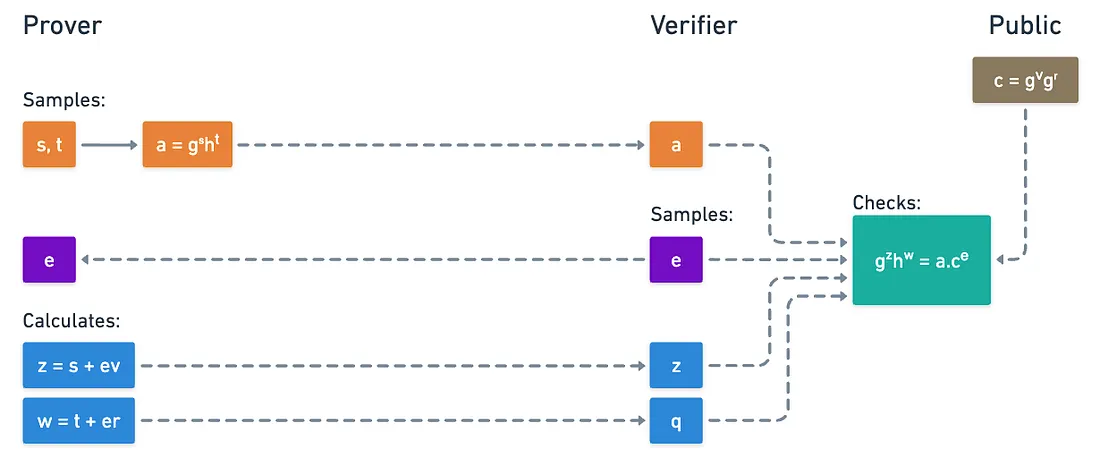
Again, the setup doesn’t take much effort: we need a group $\mathbb{G}$, generators $g$ and $h$, and the commitment $c$. All of these are completely public.

The prover secret (a.k.a. the witness) is of course the opening $(v, r)$. We proceed in the following steps:

• The prover chooses random values $s$ and $t$, and computes:

$$a = g^sh^t$$

• Upon receiving this, the verifier samples a single random challenge $e$, and sends it to the prover:

$$e \overset{\$}{\leftarrow} \mathbb{Z}_n$$

• The prover computes the pair $(z, w)$ and sends it to the verifier:

$$z = s + ev \ (\textrm{mod} \ n), \ w = t + er \ (\textrm{mod} \ n)$$

• Lastly, the verifier checks:

$$g^zh^w \overset{?}{=} ac^e$$

Click to zoom

I invite you to check for completeness and soundness (maybe even special soundness) for yourself!

And when you check for completeness, you’ll in fact be using the additively homomorphic properties of Pedersen commitments: the commitment to the values $(z, w)$ can be derived homomorphically from the commitments to the individual values!

What’s cool about this is that the Okamoto protocol can be used anytime we have a Pedersen commitment in a cryptographic protocol, and we need to prove we know its opening without revealing it.

We could get really creative with this. There is however one particular example I want us to look at, that will be of special interest in our quest.

That, and because I made some promises around it!

Multiplication Gates

Exactly! We hit a dead end last time, because unlike addition gates, multiplication gates did not fare too well with Pedersen commitments.

We promptly noted that the commitments themselves are not proving systems. But now, armed with the notion of Sigma protocols, perhaps that is something we can do!

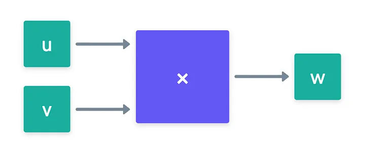
The problem requires a slightly different framing though, so let’s start there. Imagine we have three values that correspond to the two inputs and the output of a multiplication gate. Our goal is to prove these values satisfy said relation, but without revealing them.

Click to zoom

To hide these values, we first commit to them, using of course our trusty Pedersen commitment scheme:

$$c_a = g^ah^{r_a}, \ c_b = g^bh^{r_b}, \ c_c = g^ch^{r_c}$$

Multiplying commitments doesn’t work any longer, but remember: all we need is to prove the values satisfy the relation! So, we’ll use the Okamoto protocol, along with a little extra.

It goes:

• The prover samples five random values $s_1$ through $s_5$. For the first four, they commit them normally:

$$\alpha = g^{s_1}h^{s_2}, \ \beta = g^{s_3}h^{s_4}$$

• The last commitment is slightly different: instead of using generator $g$, we swap that by the commitment to $a$ (just trust me for a moment, I promise things will cancel out nicely later):

$$\gamma = c_a^{s_3}h^{s_5}$$

• Then, the verifier sends the usual challenge $e$.
• The prover calculates a total of five responses. The first four are quite straightforward:

$$z_1 = s_1 + ea, \ z_2 = s_2 + er_a, z_3 = s_3 + eb, \ z_4 = s_4 + er_b$$

• But the last one is a little different:

$$z_5 = s_5 + e(r_c {-} r_ab)$$

• With this information, the verifier is ready to perform their checks.

So what checks should they execute? Evidently, they can validate knowledge of $a$ and $b$ using exactly the same recipe from the Okamoto protocol:

$$g^{z_1}h^{z_2} \overset{?}{=} a{c_a}^e, \ g^{z_3}h^{z_4} \overset{?}{=} b{c_b}^e$$

No surprises here. What can we do about $c$ though?

This:

$${c_a}^{z_3}h^{z_5} \overset{?}{=} \gamma {c_c}^e$$

What?

Breathe, just breathe. Let’s take it step by step.

We must check this by expanding the expressions. Starting on the left side, and assuming of course $c = a \cdot b$:

$${c_a}^{z_3}h^{z_5} = (g^ah^{r_a})^{s_3 + eb}h^{s_5 + e(r_c {-} r_ab)} = g^{a(s_3 + eb)}h^{r_a(s_3 + eb) + s_5 + e(r_c {-} r_ab)}$$ $$= g^{as_3 + eab}h^{r_as_3 + r_aeb + s_5 + er_c {-} er_ab} = g^{as_3 + ec}h^{r_as_3 + s_5 + er_c}$$

And now we start grouping things together:

$$= (g^{a})^{s_3}(h^{r_a})^{s_3}(g^{c})^e(h^{r_c})^eh^{s_5} = {c_a}^{s_3}h^{s_5}{c_c}^e = \gamma {c_c}^e$$

Just like magic, we arrive at the expected expression! What kind of sorcery is this?

The key to this matter is in a surgical cancellation, courtesy of the way we defined $z_5$. It wasn’t a fluke: it has to do with the fact that, when $c = a \cdot b$, we can play around with the commitment to $c$, by using a centuries old-trick: multiplying by $1$, and expressing that $1$ in a convenient way. Here:

$$c_c = g^{c}h^{r_c} = g^{ab}h^{r_ab}h^{r_c}h^{-r_ab} = {c_a}^bh^{r_c-r_ab}$$

Ahá! Check out that last exponent! It sure looks similar to $z_5$.

What happens is that we can interpret the commitment to $c$ in an alternative way: as a commitment to $b$, using generators $c_a$ and $h$, and a very specific randomness that acts as the correction term. Combined with the commitment $\gamma$, and with appropriate commitment manipulation, everything lines up perfectly.

And so, the method is complete.

I’ll once again skip the soundness demonstration to keep things brief, but you can try it yourself if you so wish to!

In short: by cleverly reinterpreting commitments and using Sigma protocols, we can prove that three hidden values satisfy $c = a \cdot b$ without ever revealing them. Nice!

Circuits

At this point, we’ve accumulated quite the toolbox. We have a way to prove knowledge of openings for a multiplication gate, and if you think about it, the Okamoto protocol in its basic form would work for addition gates.

Although the homomorphic properties of Pedersen commitments should be enough to work with those!

Huh... But if we can treat both gate types, can we not deal with full arithmetic circuits? Could we not prove all gates are correct simultaneously?

Yes! If we commit to each wire, a verifier could easily work their way through addition gates (in fact, we don’t need to commit to the output of addition gates), and we can use a separate Sigma protocol for each multiplication gate.

It’s a noble idea... And one with an obvious problem. The strategy scales poorly as the number of multiplication gates increases, which translates into an increasing number of required communication steps.

Or into a larger proof size, when applying the Fiat-Shamir transform.

Not everything is lost though, as we can mitigate this through a cool trick: composition!

Composition

Composing claims together means that we can check two or more openings at the same time. And there are two flavors for this: we prove knowledge of both statements (AND composition) or we prove knowledge of either statement (OR composition).

Of course, in OR composition, the idea is not to reveal which statement we have knowledge of!

For circuits in particular, what we need is to prove knowledge of all the commitments of all multiplication gates, all at once. That’s exactly the idea of AND composition. So how do we do that?

The trick to this is surprisingly simple: instead of running separate protocols with different challenges for each gate, we use a single shared challenge $e$ for all of them!

Concretely, we’d have the prover sends all commitments ($\alpha$, $\beta$, and $\gamma$ for each multiplication gate), and the verifier would send one challenge $e$ in response. The prover responds to all gates using that same $e$, and verification happens under this same assumption.

And it’s perfectly safe to do this: a cheating prover would still have to guess the value, so this is as hard as before!

Thus, we can handle the entire circuit in a single commit-challenge, response cycle!

OR composition, on the other hand, is not very useful for our purposes. Yet, it can be a strong foundation for things like ring signatures and anonymous credentials.

It’s all good and dandy until we realize that circuits can have a very large number of multiplication gates.

This is problematic for a minor detail I didn’t mention: the number of commitments scales linearly with the number of multiplication gates. And linear scaling is not the best: a circuit with millions of gates will require sending a number of commitments and field elements also in the order of the millions.

So, yeah... We’ve hit another brick wall.

Despite being technically possible, this alternative is not really practical for large circuits. And in order to produce more manageable proofs, several optimizations are applied by more advanced systems.

Summary

Oh wow. That was a lot.

My brain feels like mush after writing all this, so I can imagine you’re also tired. But hey! We covered a lot of ground today.

Sigma protocols are super useful. They can even be used as subprotocols of more complex constructions. And I reckon I framed composition in a somewhat pessimistic manner, but it really is a nice tool to have, especially when we’re dealing with a small number of commitments.

Importantly, we successfully applied our newfound knowledge of groups to build a new kind of protocol.

Given their simplicity, we'd be forgiven to think that there’s not much we could do with groups. And that could not be further from the truth.

Especially because of those optimizations I mentioned before. I don’t want to spoil the fun, but to give you a small hint, this has to do with how we encode circuits.

Instead of thinking about circuits as collections of individual gates, and instead, reinterpret them as something we haven’t talked about for a while now: polynomials!

You thought we were done with them? Ha!

And instead of checking millions of individual constraints, the verifier can check a few polynomial identities, and be done with the whole thing!

Working with polynomials efficiently relies on a single algorithm — and this algorithm has everything to do with groups.

Therefore, before we continue with more advanced proving systems, we’ll need to make a strategic stop to understand this mechanism, which is nothing short of one of the most important and elegant algorithms mankind has ever developed.

Join me in the next one to find out what it’s all about!