---
title: 'Understanding AI: Regression'
description: >-
We put our three pillars to work on linear regression, uncovering why squared
errors make sense through Gaussian noise and likelihood, and how a plain line
can learn to fit curves.
author: Frank Mangone
date: '2026-11-16'
lang: en
series: understanding-ai
tags:
- artificialIntelligence
- machineLearning
- mathematics
- optimization
- regression
- probabilityAndStatistics
url: 'https://arkana.blog/en/blog/understanding-ai/regression/'
---
# Understanding AI: Regression
Thanks to the previous [two](https://arkana.blog/en/blog/understanding-ai/an-introduction) [articles](https://arkana.blog/en/blog/understanding-ai/humble-beginnings), our mental model to understand the moving parts of ML should be more or less established: vectors and linear algebra for **representational purposes**, probability and statistics as the framework behind **naturally uncertain data**, and optimization as the technique that ultimately allows us to **flesh out good predictors**.
And I know we've been working at a somewhat abstract level so far, without really applying most of the concepts we've learned. So how about we take a stab at **seeing them in action**?
To really kick off our journey then, we'll begin by looking at arguably the simplest kind of predictors we can find: **linear models**!
> Remember that, as we discussed [a couple articles back](https://arkana.blog/en/blog/understanding-ai/an-introduction#models), there's a wide range of models we could choose from, ranging from very plain and simple ones, to very sophisticated and complex. Choosing the right model for the task at hand will usually be our first challenge!
It's a deceptively big family of models, and today we'll only zoom in on its most iconic member: **linear regression**. A very simple model, with a ton to learn from.
Sounds like a plan then! Where do we start?
---
## Linear Regression
Our first mission is very simple: we'll try to fit some data to a plain ol' **line**.
I know, I know - you're here for all the AI goodness, and here I am, trying to draw a line through some points.
> Yeah, what the hell dude.
Before you abandon ship though, let me just say this: linear regression has a **lot** to teach us about things that we'll be using even in the most complex of settings. And despite its apparent simplicity, there are **entire books** (like [this one](https://www.kwcsangli.in/uploads/3--Introduction_to_Linear_Regression_Analysis__5th_ed._Douglas_C._Montgomery__Elizabeth_A._Peck__and_G._.pdf) or [this one](https://www.stat.purdue.edu/~qfsong/teaching/525/book/Weisberg-Applied-Linear-Regression-Wiley.pdf), just to name a couple) solely dedicated to analyzing this humble little guy. So yeah, it's a much deeper topic than one would imagine.
Assuming you're still there (I really hope so), let's start by framing our problem first, and then we'll see how we can handle ourselves around it.
### Drawing Lines
Back in my days as a chemical engineering student, linear regression was a tool we used quite often (though never under the branding of Machine Learning). As it turns out, many observations about the physical world are either simple linear relations, or can be cleverly manipulated to behave as such. So the simple act of drawing lines became a fundamental tool for analysis, and has allowed scientists throughout history to pinpoint physical constants and validate mathematical laws to describe the world.
> I'd say those credentials are hard to ignore, even when you cannot chat with a line!
But rather than drawing these lines by eye, we'd like to apply the things we learned in the [previous article](https://arkana.blog/en/blog/understanding-ai/humble-beginnings) in a methodical way. And for that, we first need to ask ourselves: just **what is a line**?
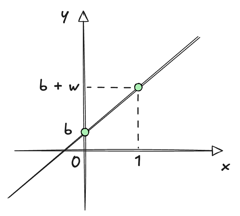
Yes, I know you know what a line is. However, we need more than an intuition: we need a precise mathematical representation that we can work with. In its simplest form possible, said representation is just a **function** of this form:
$$
\ell: f(x) = w \cdot x + b
$$
As you can see, this little guy has only **two parameters**; two little knobs we can adjust.
The first one is usually called the **slope** $w$, and controls how steep the line is. The bigger the slope, the faster the output will grow (or shrink) as we move the variable $x$. The second one, normally called the **intercept**, controls where the line sits **vertically** on a plane. It's the value we get when $x$ is exactly zero, so it serves as our "starting point" of sorts.
Now, naming conventions are not always the most obvious in math, and we sometimes use weird letters to represent quantities. Even then, the choice of $w$ and $b$ for the slope and intercept in this case is not a decision made on a whim, but in fact **quite deliberate**.
In the world of Machine Learning, these two quantities receive **special names**. You might have already guessed what $w$ stands for, since we've already talked about it: we call it the **weight**, and it relates to how sensitive our model is to changes in the variable $x$.
The other one, we call the **bias** $b$, and it's exactly that: how skewed or biased our model is when weights don't matter, meaning the value of $x$ is either 0 or close to it.
> You could think of this as the "default value" of the model. And mathematically speaking, this is the knob that allows us to avoid having the line go through the origin $(0,0)$.
These names will follow us for the rest of the series, so using $w$ and $b$ is a good reminder of what these thingies mean. When we get to fancy things like neural networks, we'll find that they're really just a whole lot of weights and biases stacked together and transformed in interesting and convoluted ways, so getting acquainted with them early will pay off big time later!
Lastly, there's one extra piece of notation worth introducing before we move on. Our simple line spits out a **prediction**, and as you might remember from our discussion about uncertainty, a prediction is just a **guess**. To make this very clear, we'll assign a special notation to predictions:
$$
\hat{y} = w \cdot x + b
$$
Anything with a little hat on top, unless stated otherwise, is a prediction - and we'll reserve the $y$ notation for the actual observed values (the ones we'll try to match as best as possible).
---
With that, we have our model, a harmless little line. But we haven't said anything about the specific values of $b$ and $w$. After all, there are **infinitely many** lines to choose from, each with its own parameters.
Obviously, we're interested in a **single line**, the one that best fits our data. Which begs the question: **how do we find it**?
### The Loss Function
We've already outlined how the usual process goes in our previous encounter. Since we now have an actual model, our next step is to choose a **suitable loss function**, and minimize its value by adjusting the model's parameters ($w$ and $b$).
But... how do we know **what a suitable loss function is**?
It's a tricky question. A loss function must measure how wrong the prediction is, but the thing is there are also **infinitely many ways to go about this**! So I guess we should start with what feels more **intuitive**, and see where that takes us.
Perhaps the simplest way we could measure "wrongness" is by calculating an **error** for each prediction, and then we just add those errors up. Something like:
$$
e_i = y_i - \hat{y_i}
$$
And then just:
$$
\mathcal{L}(w, b) = \sum_{i=1}^n (y_i - \hat{y}_i(w,b,x_i))
$$
There we go. Lookin' good. This should work, right?
Well think again! There's in fact a **huge problem** with this loss function.
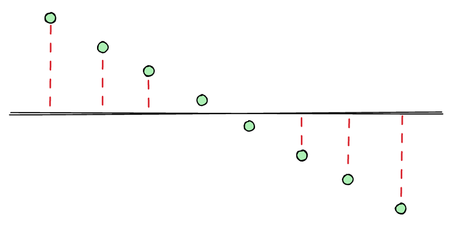
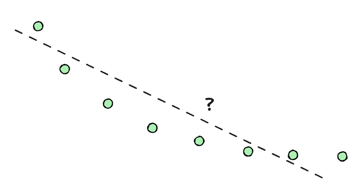
The issue is that the **sign** of the errors matters. Some errors might be positive, and some might be negative, so they could **balance out** even when a simple visual inspection would tell us some line makes **absolutely no sense**! For example, the horizontal line here is a terrible fit (and it's pretty easy to spot the actual trend), but the errors would cancel out, giving a loss function value very close to $0$:
This won't do. At least not in its current shape... but maybe we can **refine** our loss function a little bit more.
All we need to do is find a way for the errors to **never cancel out**, and that should do the trick. And while there are also many ways to do this, one strategy reigns supreme in this area: squaring the errors!
$$
\mathcal{L}(w, b) = \sum_{i=1}^n (y_i - \hat{y}_i(w,b,x_i))^2
$$
By doing this, all the terms will be **positive**, so the loss function will always take non-negative values, and the errors will never cancel each other out.
Alright, that looks like a much finer choice! For now at least, we'll run with this so-called **sum of squared errors** loss function.
> The fact that it gets its own name should be indicative of its importance (wink, wink). We'll analyze this in detail further down below.
>
> You'll often see this divided by the number of points $n$, which gives the **mean square error** (or **MSE** for short). Since $\frac{1}{n}$ is just a constant, the best $w$ and $b$ come out exactly the same, so we'll stick with the plain sum.
### Finding the Best Fit
Naturally, the next step is to find the parameters $w$ and $b$ that produce the **best fit**, meaning that they **minimize the loss function**.
With this model, it's actually possible to do something we'll almost never be able to do: finding a **closed form** solution for the best parameters. In other words, an **explicit formula**.
We'll do this by finding the minimum of the loss function, only that... we still don't know how to do that! Luckily for us, finding it is very straightforward, as everything relies on a very simple fact about minima (or maxima).
> Just in case, **minima** and **maxima** are the Latin plurals of **minimum** and **maximum**. Which you can use for extra fancy points, although minimums and maximums are also acceptable.
Remember the [slope of a multidimensional hill](https://arkana.blog/en/blog/understanding-ai/humble-beginnings#an-extra-requirement) we talked about last time? Well, a minimum (or a maximum) will sit at a point where there's exactly **no slope**. Which makes sense, right? We go down and down until there's no more slope to walk down in any direction we look at!
Great. That gives us a set of conditions (usually called first-order conditions) that a minimum should satisfy:
$$
\frac {\partial \mathcal{L}}{\partial w} = 0 \qquad \frac {\partial \mathcal{L}}{\partial b} = 0
$$
After we calculate the derivatives and simplify a bit, we end up with two expressions:
$$
\begin{gathered}
\sum_{i=1}^n x_iy_i = w\sum_{i=1}^n x_i^2 + b\sum_{i=1}^n x_i \\
\\
\sum_{i=1}^ny_i = w\sum_{i=1}^n x_i + n \cdot b
\end{gathered}
$$
Which look scary, until you realize those big sums are just numbers we can calculate from our observations, and that there are only two unknowns, $w$ and $b$.
It's a system of two equations for two unknowns, so if my high school memories serve me right, we should be able to solve this! From this point on, it's just a little more algebra (that I'm gonna conveniently skip in the interest of keeping this brief), and we arrive at the closed-form results we're looking for.
> For simplicity, we need to introduce the **average** of all $x_i$ values as $\bar{x}$, and likewise $\bar{y}$ for the $y_i$ values. But remember, these are just values we can calculate directly!
$$
\begin{gathered}
w = \frac{\sum_{i=1}^n (x_i - \bar{x})(y_i - \bar{y})}{\sum_{i=1}^n (x_i - \bar{x})^2} \\
\\
b = \bar{y} - w\bar{x}
\end{gathered}
$$
And voilà! Those are the optimal $w$ and $b$! Piece of cake, right?
> While we don't need to worry about analyzing these results too much now, I'm gonna say a couple things for those of you who might be interested in a bit more, because there's a lot to unpack even for such a simple model.
>
> If you happen to have some more context on probability, notice that $w$ is really just the **covariance** between $x$ and $y$, divided by the **variance** of $x$. That means $w$ is a measure of how much $y$ tends to move together with $x$, scaled by how spread out $x$ is. And $b$ simply anchors the line so it passes through $(\bar{x}, \bar{y})$, sort of the "center of mass" of our data.
>
> We'll talk more about variance and covariance in due time, but the ideas are simple enough they allow us to at least make **some** sense out of the result.
While this can be done fairly easily with a few operations from linear algebra (namely a couple matrix multiplications), I think it's fair to say this whole process is a bit tedious. And things will only escalate from this point onwards... so do we really have to go through such a painstaking process every time?
To properly answer that, I'd first like for us to use our little formulas to "train" our first model.
Shall we put it to the test then?
### A Worked Example
I'm just gonna say this once: I absolutely despise Python. You know who likes it though? The entire freakin' data industry, that's who!
> Like, seriously, everyone and their mother uses it.
So in the name of convenience and convention, the examples we'll be working through along the way will all be in Python. I'll ask you in advance to excuse my non-fluency in the language. You can probably do it cleaner and better - just bear in mind these are mere examples.
> Oh, and by the way, the code blocks below are **live**: press **Run** (or Shift+Enter) to execute them right here in your browser, and feel free to edit them and see what happens. They all share a single session, so if you run a block that depends on earlier ones, those will run first.
Okay then! Let's start by generating a few points around a line:
```python
import numpy as np
rng = np.random.default_rng(42)
n = 40
true_w, true_b = 2.5, 1.0
x = rng.uniform(0, 10, n)
y = true_w * x + true_b + rng.normal(0, 2, n)
print(f"Generated {n} points around y = {true_w}x + {true_b}")
print(f"-----------------------------------------------------")
print(f"First three points:")
for xi, yi in zip(x[:3], y[:3]):
print(f"x = {xi:.2f}, y = {yi:.2f}")
```
Nothing fancy: we're just picking a "true" line (initially $w = 2.5$, $b = 1$, but you can change those values) and generating some points around it, with a bit of random noise (we'll talk more about that in a second) thrown in to make things a little more realistic. If we plot these points, we get:
```python
import matplotlib.pyplot as plt
# Uses x and y from the cell above
plt.scatter(x, y)
plt.xlabel("x")
plt.ylabel("y")
plt.show()
```
A nice, noisy cloud of points, showing a clear linear trend. Now, let's put those closed-form formulas we derived earlier to work, and see if we can recover something close to our original line:
```python
# Uses the data and imports from the cells above
x_mean, y_mean = x.mean(), y.mean()
w = np.sum((x - x_mean) * (y - y_mean)) / np.sum((x - x_mean) ** 2)
b = y_mean - w * x_mean
print(f"w = {w:.2f}, b = {b:.2f}")
# Sorted, so the lines are drawn left to right in a single pass
xs = np.sort(x)
y_true = true_w * xs + true_b
y_pred = w * xs + b
plt.scatter(x, y, label="data")
plt.plot(xs, y_true, color="teal", linestyle="--", label="true line")
plt.plot(xs, y_pred, color="magenta", label="fitted line")
plt.xlabel("x")
plt.ylabel("y")
plt.legend()
plt.show()
```
Pretty close, huh? Sure, we don't get a perfect match, but it's **close enough**. It's reasonable to say our little formula has done its job.
But there's an important lesson to take away from this: even with our exact formula, found by deriving the equation for the optimal solution, we still didn't recover the **real model**. We never really do, because as we've mentioned many times already, **real data is noisy**.
So to answer the question from before: do we really need to find those closed-form formulas for the optimal solution given the loss function we're using? **Not really**! There are other, simpler ways to get to a **good enough solution** - and if we do that carefully, good enough might as well be as close to reality as the actual optimal solution, because the latter isn't perfect anyway!
> In short: since we're always dealing with imprecise data, "good enough" is probably okay. We still need to measure what that means (we'll get there, I promise), but we should be at peace with the idea that no model will ever be perfect.
---
Wonderful! We've officially "trained" our very first model. Not bad, eh?
> And believe it or not, this simple artifact is used absolutely everywhere out in the wild. Economists use it to estimate how spending affects growth. Doctors use it to relate dosage to blood pressure. Real estate sites use it to guess a house's price from its size and location. Any time there's a rough "as $X$ goes up, $Y$ tends to go up (or down) too" kind of relationship lurking in some data, there's a good chance a straight line is quietly doing the heavy lifting behind the scenes.
Trust me, there is **a lot** more to say about this model, innocent as it may look. We could talk about how to measure how well the line matches the data, or about what to do when one point seems to tell a different story than the rest.
Those will be topics for another day. Alas, there are two loose ends I'd like to tie up before moving on, because both will follow us for the rest of the series.
---
## Why Squares?
The first question has to do once again with our loss function of choice. We chose to square the errors, and things worked out quite nicely... but was it just pure coincidence, or was our loss function actually part of that success?
If you recall, our only requirement was that errors should **never cancel out**. Squaring them did the job, but taking their **absolute value** would have worked just as well (for that purpose, at least). So is there anything special in choosing squares?
Well, there are actually two reasons for this. The first one is quite mundane: mathematical convenience. Squares are easy to work with when derivatives are involved, so they make calculations very manageable.
The second reason is a bit more involved, but well worth the effort. And we'll take this chance to introduce yet another acquaintance that we'll need in our journey.
> Not gonna lie, this next part will be a bit dense. I would advise not to skip it though, since it introduces some important ideas.
>
> If you feel a little stuck as you read this section, I suggest jumping straight into [Beyond Straight Lines](https://arkana.blog/en/blog/understanding-ai/regression#beyond-straight-lines), and maybe coming back later.
Let's think about our [dice example](https://arkana.blog/en/blog/understanding-ai/humble-beginnings#probability-statistics) from the previous article. Remember how as we added more and more dice, the tiny noise contributions from each individual die added up in a very particular pattern, which looked like a bell.
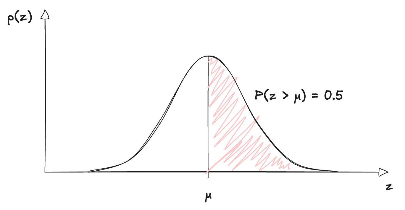
That was no coincidence either. Perhaps mysteriously, this distribution appears in all sorts of unrelated phenomena. It's so common that it gets a very particular name, one you've probably heard before: the **normal distribution** (also known as **Gaussian distribution**).
> a.k.a. the famous bell curve.
In its general one-dimensional form, the normal distribution is described by this formula (I'm using $z$ for the variable so that we don't mix things up with our input $x$):
$$
p(z) = \frac{1}{\sqrt{2\pi\sigma^2}} \exp\left(-\frac{(z - \mu)^2}{2\sigma^2}\right)
$$
There, there. Yes, I know it looks scary. But trust me, it's not that bad once we start unpacking it. Here, let's do it together, slowly. First, the left-hand side: what's that $p(z)$?
When we roll a die, each of the six outcomes had a probability of $1/6$. But measurement errors do not behave like a die roll - instead, they are a **continuous** quantity that can take **infinitely many values**, so the chance of landing on one exact value is essentially **zero** (because we have infinitely many other possibilities).
Thus, instead of assigning probabilities to **single values**, we describe the distribution with a **density**: the height of the curve $p(z)$ tells us how plausible the values **around** $z$ are, compared to others. The higher the curve, the more plausible.
And the probability of landing **between any two values** is the **area** under the curve between them. The total area is exactly $1$, which is the same rule we had before: all probabilities must add up to $1$, which translates to $z$ having to **land on some value**!
> You'll also see this density written as $f_Z(z)$ in other texts, particularly in statistics books, where the subscript tells us which [random variable](https://en.wikipedia.org/wiki/Random_variable) the density belongs to. Same thing, different notation. We'll stick with $p(z)$, as it's the more common choice in ML textbooks.
Then, there are two numbers that control the **shape** of the bell:
- $\mu$ is called the **mean**, and sets the **center**: the curve peaks right there, and falls off symmetrically on both sides.
- $\sigma$ is called the **standard deviation**, and sets how **spread** the curve is. The bigger the spread, the wider and flatter the bell.
> Its square, $\sigma^2$, is the **variance** we mentioned before. No need to dwell on the details for now though.
So these are exactly the **center** and **spread** we talked about last time, now with proper names! And since this distribution will keep popping up, we'll write it in a handy shorthand form:
$$
z \sim \mathcal{N}(\mu, \sigma^2)
$$
Which reads "$z$ follows a normal distribution with mean $\mu$ and variance $\sigma^2$".
Finally, look at what's inside the exponential: $(z - \mu)^2$, the **squared distance** from the center. The farther $z$ is from $\mu$, the smaller the density gets. Keep that squared distance in mind, because it's about to become very important!
### Gaussian Errors
Ok, cool... but what does all of this have to do with our loss function?
Back to our noise it is. Noise is something we **don't get to choose**: it's just there, in the data. What we can do is make an **assumption** about how it behaves, which is just another way of saying we **model** it. And thanks to our dice, we have a very good candidate: lots of tiny, independent nudges add up to a bell shape. So we'll assume the noise in each observation (which we'll call $\varepsilon$) follows a **normal distribution**, **centered at zero**:
$$
\varepsilon \sim \mathcal{N}(0, \sigma^2)
$$
Centering it at zero means we're assuming noise has **no preferred direction**: on average, it doesn't push observations up or down.
> And any constant push in one direction would be indistinguishable from a different bias $b$, so there isn't much to gain by letting the center be anything other than 0!
If you squint a little, you'll see this is actually how our dataset came to be! Here, a little refresher:
```python
true_w, true_b = 2.5, 1.0
x = rng.uniform(0, 10, n)
y = true_w * x + true_b + rng.normal(0, 2, n)
```
Or, in math notation:
$$
y_i = w x_i + b + \varepsilon_i
$$
That means each $y_i$ is the true line's value, plus a **little bit of Gaussian noise**. Adding the line's true value just slides the center of the bell from $0$ to $w x_i + b$, so we can say that the distribution for $y_i$ should look like this:
$$
y_i \sim \mathcal{N}(w x_i + b, \sigma^2)
$$
In other words, each $y_i$ is a bell curve **centered on the line's prediction**. And that comes with a catch: the center depends on $x_i$, $w$ and $b$, so the distribution of $y_i$ **isn't one fixed thing**. It **changes** depending on those values!
As always, we need to put that in math notation, and probability has a standard way to do it: the vertical bar $\mid$. It's formally called **conditional probability**, but you can just read it as "**given these conditions**".
> To see it in action, think of a die again. The chance of rolling a six depends on whether the die is fair or loaded, so we'd say it's $1/6$ **given a fair die**, but much higher **given** a loaded one. Whatever sits after the bar is what we're taking as known information.
>
> It's a tiny piece of notation, but it goes a long way, and we'll be seeing it over and over from now on!
So for our line, we write $p(y_i \mid x_i, w, b)$ for the plausibility of seeing the value $y_i$, **given** that the input was $x_i$ and the line has parameters $w$ and $b$. And if we plug $z = y_i$ and $\mu = w x_i + b$ into the general formula, we get:
$$
p(y_i \mid x_i, w, b) = \frac{1}{\sqrt{2\pi\sigma^2}} \exp\left(-\frac{\big(y_i - (w x_i + b)\big)^2}{2\sigma^2}\right)
$$
Take a moment to see what this is telling us. If a point sits right on top of the line, the exponent is close to zero, and the plausibility is as high as it gets. If it sits far away, the plausibility drops very fast. In other words:
> Lines that pass close to the data make the data plausible, and lines that pass far from it make it look like an accident.
> Now's a good moment to take a little breather. I know this might seem like a lot, but the payoff is amazing, I promise!
### Maximum Likelihood
That suggests a different way of finding $w$ and $b$: choose the line that makes the observed data **as plausible as possible**! And to do that, we once again need a **single score** for the entire dataset, which we can then try to make **as big as possible**.
If we assume each observation is independent of the others (say, one movie rating doesn't influence the next), the plausibilities simply **multiply**:
$$
\text{Lik}(w, b) = p(y_1, \dots, y_n \mid x_1, \dots, x_n, w, b) = \prod_{i=1}^n p(y_i \mid x_i, w, b)
$$
This quantity is called the **likelihood** of the parameters, and it's a really important one. It's the probability (or, for continuous values like ours, the probability density) of the **observed data**, seen as a function of the **parameters**.
> This is also normally written as $\mathcal{L}$, but we've already claimed that letter for the loss function! As you'll soon see though, they end up being very closely related anyway.
It's worth pausing on this definition, because it's easy to mix up with plain probability:
- With **probability**, the parameters are fixed, and we ask how likely different data are.
- With **likelihood**, we flip it around: the **data** is fixed (it's what we actually observed), and we ask how well different parameters explain it.
> And despite the similar names, the likelihood is **not** a probability distribution over the parameters: it doesn't add up to $1$. It's just a score, telling us how well some parameters explain what we observed.
Choosing the parameters that make this score as big as possible is called **maximum likelihood estimation**, or **MLE** for short.
And finally, here comes the payoff: if we go ahead and find the parameters that maximize this likelihood, we end up with... drum roll please...
> Minimizing the sum of squared errors!
The algebra is short, and you can work it out yourself with pen and paper in a couple minutes (we take a logarithm so that the product becomes a sum, and the rest falls into place shortly after). The reason why this happens hides in plain sight: remember that squared distance inside the exponential? That's **exactly where our squares come from**.
In other words:
> Minimizing squared errors gives us the maximum likelihood estimate, provided the noise is Gaussian.
Therefore, using squares isn't an arbitrary choice after all! Our humble loss function had been quietly encoding an assumption about **noise** all along. And that's actually a general idea: **choosing a loss function is really choosing a noise model**. Had we assumed a different kind of noise, we'd have ended up with a different loss.
> I told you there was a lot to dig up!
> Anyway, here's a [great video](https://www.youtube.com/watch?v=WCP98USBZ0w) that provides yet another explanation of this entire thing. Maybe seeing it in motion will help cement the idea!
---
## Beyond Straight Lines
Now for the second loose end (and this will be a bit shorter, I promise): what do we do when the data simply **refuses to follow a straight line**?
What do I mean by this, you ask? Well, here's a cloud of points for you. Would you say a line is the correct predictor for them?
Probably not! No matter how carefully we choose $w$ and $b$, a straight line can't bend to follow that curved trend.
But before we throw linear regression out the window, let's take a closer look at what our model really is: a weighted sum of **features**. We just happened to choose $x$ as our only feature (and a constant $1$, to which we assign the bias).
Who said those features have to be the raw input $x$? What if we hand the model a **second feature**, like $x^2$?
$$
\hat{y} = w_2 x^2 + w_1 x + b
$$
That's no longer a line, but a **parabola**!
From the model's point of view though, **nothing has changed**. It's still a weighted sum of features - a dot product between the weights $[w_2, w_1, b]$ and a feature vector $[x^2, x, 1]$. All we did was **transform the input** before feeding it into our model, but the model itself remains exactly as linear as before, because it's **linear in its weights**.
> That's the real meaning of the word "linear" in "linear models". It says nothing about the shape of the curve we get as a function of $x$: it only says that the weights enter the formula by multiplying and adding.
>
> It's also why everything we did keeps working. The loss is still a nice bowl-shaped function of the weights, and setting its derivatives to zero still gives us a system of linear equations to solve.
Same machinery, new shape! And we're not limited to powers of $x$: we could feed the model logarithms, square roots, products of different features... pretty much anything we can compute from the input.
For example, take the famous [Arrhenius equation](https://en.wikipedia.org/wiki/Arrhenius_equation) from chemistry:
$$
k = A e^{-E_a/RT}
$$
Plotting $k$ against $T$ gives a curve, but if we take logarithms:
$$
\ln k = \ln A - \frac{E_a}{R}\cdot\frac{1}{T}
$$
Then that's a **perfectly good line** in terms of $1/T$!
---
In fact, we're not even limited to a **single input variable**. Our movie recommender, for instance, had two features: runtime and average rating. A linear model can take as many as we like, and it's the very same weighted sum we met last time, plus a bias:
$$
\hat{y} = \textbf{w} \cdot \textbf{x} + b = w_1 x_1 + w_2 x_2 + \dots + w_d x_d + b
$$
With one variable, the model draws a line. With two, a **plane**. With more, a higher-dimensional version of the same thing. And we can mix and match as we please: raw variables, squared ones, products between them... as long as the weights enter by multiplying and adding, we're still in **linear territory**.
Fantastic stuff for such a simple model, eh? Alas, before we get too excited, a word of caution: there's a little catch that can make or break the success of the model.
Importantly, **we** are the ones choosing the features here. We looked at the data, decided a parabola was a good idea, and added $x^2$. If we pick too few features, the model won't capture the pattern. But if we pick **too many** (say, we keep adding $x^3$, $x^4$, and so on), the curve will gladly wiggle through every single point, **mistaking noise for a pattern**.
We already mentioned this: **flexible models can latch onto noise**, so we end up with a small loss value, but **poor predictors**.
Finding the right balance is a recurring theme in Machine Learning, and we'll come back to it time and time again. And as we'll see further along our path, one of the great ideas behind neural networks is that they **learn good features on their own**, rather than relying on us to guess them.
---
## Summary
I bet you wouldn't have imagined there was so much to say about a humble line!
Today, we saw our first proper model in action, **linear regression**. It was a great exercise in problem framing and loss function selection, and we even found a **closed-form solution** for the **best possible** weight and bias!
Along the way, we picked up two important ideas that should stick with us:
- The first is **likelihood**: the probability of the observed data, seen as a function of the parameters. Maximizing it under Gaussian noise turned out to be the same as minimizing squared errors, which tells us that a loss function can hide an implicit assumption about **noise**.
- The second is that "linear" means **linear in the weights**, so by feeding the model non-linear **features**, a plain linear model can fit curves too.
> Remember, this is all about building the **foundations**. We'll get to the cooler stuff once we've cleared the basics!
---
And there's another thing we must ask ourselves before we go: what kind of question did our model actually answer?
You see, regression spits out a **continuous output**: a number that can take any value along a certain range. That's just what we need to pin down something like a physical value, or to estimate a house's price.
But think back to our recommendations engine from the [start of the series](https://arkana.blog/en/blog/understanding-ai/an-introduction#an-examination-of-data). Suppose a line predicts that Alice would rate a certain movie a $6$. Does that mean she'd **like** it? What about a $4$? Who the hell knows!
What our engine really needs is something even more humble: a simple **yes** or **no**. That's a different kind of problem, called **classification**, and along with regression, it's one of the **two big families** that most of the machine learning techniques we'll meet are built around.
So how do we go about it? We'll see that, curiously enough, **drawing lines** can still help us out. But we'll also ask ourselves whether geometry is the right way to think about the problem to begin with, and that's where probability (and our new likelihood gadget) comes back into play.
That's exactly where we'll be headed next. See you soon!
## Key concepts
### Weights and biases
A line is a model with two knobs: the **weight** $w$ (slope) and the **bias** $b$ (intercept). Predictions wear a hat: $\hat{y} = w \cdot x + b$.
### Squared errors
Plain errors can **cancel out**, so we square them before adding. The result is the **sum of squared errors** loss (divide by $n$ and you get the **MSE**).
### Good enough fits
For a line, setting the derivatives to zero gives a **closed-form** solution for $w$ and $b$. But noise means we never recover the **true** line, so a good enough fit is fine.
### Likelihood
The **likelihood** is the probability of the observed data as a function of the parameters. With **Gaussian noise**, maximizing it is the same as minimizing squared errors: choosing a loss means choosing a **noise model**.
### Linear in the weights
"Linear" means linear in the **weights**, so feeding in features like $x^2$ lets a linear model fit **curves**. Too many features, though, and it starts fitting **noise**.
### Regression vs classification
Regression predicts a **continuous number**. Answering a **yes or no** is a different problem, called **classification**.