The ZK Chronicles: Commitment Schemes (Part 2)

Throughout the two previous articles, I’ve been hinting at how modern ZK systems rely on ways to, loosely speaking, encode circuits as polynomials.

While we don’t have the full context of how this will work yet, using this strategy will require us to design a new type of commitment scheme. We’ll no longer commit to individual values, but to the polynomials themselves.

I reckon this might sound weird at first. But this is actually something we hinted at a long time ago, back when we learned about the sum-check protocol.

Let’s flex those memory muscles a bit!

We talked about having oracle access to some polynomial back then, but we didn’t really know how to do that.

Today is the time to uncover that mystery. And with this, we’ll be all set with preparations, and fully ready to look at some protocols once again.

Ready? Let’s go!

Motivation

It’s a good idea to start by imagining how this whole “committing to a polynomial” deal will play out.

The main idea is quite straightforward, really: instead of checking all gates in a circuit, we’d like to sample some constraints at random.

For example, the wires connecting to a multiplication gate should follow the expected $a \cdot b = c$ relation. Or maybe, some wires $x$, $y$, and $z$ should have the same value.

We then want to evaluate the encoding polynomials at the positions that give us the information we need to check the desired constraint, and then we just check that the constraint is satisfied.

Sounds easy, right?

As you may have learned to expect by now, it’s never that simple. The problem in this case is that these encoding polynomials will be at least as big as the original circuits themselves... so sending these polynomials to a verifier is not much better than just sending commitments to all wires!

Like we did in our Sigma Protocols example. Remember, it wasn’t a very scalable strategy.

For this to work then, we’ll need a different approach. So here’s an idea: how about we avoid sharing the polynomial altogether?

Essentially, we could try to devise a way for a verifier to request evaluations. This is the setup we originally called oracle access to a polynomial: you don’t calculate evaluations yourself, but rather defer the workload to a trusted party.

Trust, however, is a word we must use with caution. And in the case of a prover trying to convince a verifier, simply trusting the former to deliver correct evaluations is a recipe for disaster.

Because it would open the cheating floodgates!

So really, what we’re after is a way to request verifiable evaluations: I ask for the evaluation of some polynomial $P(X)$ at some value $a$, you compute it, but not only do you respond with $P(a)$, but also with a little proof of validity or correctness.

This is the essence of the commitment schemes we’ll be studying today: polynomial commitment schemes, or PCS for short. We’ll see that the proof of correctness is usually validated against an initial commitment to the polynomial in question  -  which is the reason these thingies are called commitment schemes at all.

Great! That’s just about enough preamble for us to understand where this is headed.

Let’s start simple!

Merkle Trees

The very first type of polynomial commitment scheme we’ll talk about is one we’ve already mentioned. The strategy is bulky, but straightforward: just commit to every possible functional value at once!

That’s right!

We already saw this in action: all we do is calculate a root, and then we prove inclusion via a Merkle path. Easy as pie!

Limitations

However, back when we first talked about this idea a couple articles ago, we immediately spotted a problem with the approach. We noted this is a good way to commit to a number of values, but how do we know these values actually come from a polynomial?

Indeed, Merkle trees are a great way to commit to $n$ arbitrary values, but proving they are polynomial evaluations takes a little extra effort.

The solution comes in the form of a technique called Fast Reed-Solomon Interactive Oracle Proofs (or FRI, for short).

Yeah, the name sounds scary, I know. And it’s actually quite involved, so we’ll leave the details for later, for when we see a type of proving system called STARK.

Even if it’s not necessary to go into specifics, there’s something I can tell you in advance: the best FRI can do is showing the committed polynomial has a degree lower than some upper bound $d$. That’s all we can know!

That will be enough in some contexts, but in most cases, it won’t. We’ll often need stronger guarantees, which in our case means to get exact degree bounds.

Why? Well, remember how we said we’d be encoding circuits as polynomials? The success of encoding strategy depends on a precise relationship between circuit size and polynomial degree.

It’s definitely possible to get these guarantees. But for that, we’ll need yet another piece of cryptographic machinery.

Pairings

Ever since we introduced groups into our toolkit, every single construction we’ve produced has lived in a single group. That’s completely fine, because we’ve always leveraged the discrete logarithm problem, so everything is built on top of some solid security assumption.

Alas, there’s only so much you can do with a single group.

In particular, the commitment scheme we'll be looking at further ahead is based on something we already know to be problematic: multiplying exponents. Remember, adding exponents is easy:

$$g^a \cdot g^b = g^{a + b}$$

But multiplying them? No cigar. At least, if we only consider standard group operations.

Luckily for us, there's a gadget we can use to do just this: pairings! They exist for exactly this reason: allowing us to sort of multiply elements from different groups.

It sounds like a simple task, but it’s actually extremely complex to get right. The mathematics behind them are as elegant as they are cryptic, so we won’t be diving into the inner mechanisms that make pairings possible. We only care that they exist, and that some trustworthy cryptographer has implemented a good library we can use.

However, if you really, really want to know how pairings work, I won’t stop you. It’s a wonderful topic. You can read more about them here. Although you might need to start here to grasp some important foundational concepts.

Definition and Properties

Let’s go with the definitions then. A pairing is a function or map that takes two inputs coming from different groups, and produces an output that belongs in yet another group:

$$e: \mathbb{G}_1 \times \mathbb{G}_2 \rightarrow \mathbb{G}_t$$

Not every map of this kind is a pairing, though. For it to be considered as such, it must satisfy a particular property, called bilinearity. Using our trusty exponential notation, this one can be summarized as:

$$e(g^a,g^b) = e(g,g)^{ab}$$

Essentially, bilinearity grants us the ability to move exponentiation around. And that simple reshuffling allows us to do some pretty cool things.

To make this a little more complete, I should also mention that we need these maps to be non-degenerate ($e(g, h) \neq 1$ for generators $g$ and $h$), and efficiently computable.

There you have it, that’s what a pairing is. Again, we’ll move forward under the assumption that we can find such functions.

Okay! But why are pairings so special?

Decisional Diffie-Hellman

Well, actually, their existence makes them special for the wrong reasons: they happen to break a problem that used to be considered hard.

In cryptography, this is generally not a good thing.

To fully understand the power of pairings then, we need to talk about that assumption, related to the discrete logarithm problem we know so well.

The setup looks like this: imagine we have a large group, and I give you three group elements: $g^a$, $g^b$, and $h$. The question is simple: can you determine if $h$ is equal to $g^{ab}$?

Think about it for a moment. We’re not asking whether $h$ equals $g^{a + b}$, as that would be trivial. No, we’re asking about the product of $a$ and $b$. If we know $a$ and $b$ in advance, we can do the calculation, sure. But going the other way around would require us to solve discrete logarithm problems, which as we know, are very hard to crack.

This is what we call the Decisional Diffie-Hellman problem, or DDH for short. Assuming that this problem is hard is key to the security of some popular cryptosystems, like Diffie-Hellman key exchange and ElGamal encryption.

Here’s the thing though: pairings break DDH. There are ways to create what we call a self-pairing, which uses inputs from the same group, and simply check this:

$$e(g^a,g^b) = e(g,g^{ab})= e(g,h)$$

And you get your answer.

So, if pairings break DDH... Are pairings dangerous then?

Not at all! Or at least, they would be, if they were easy to find.

Also, as a sidenote: notice how even if we’re able to break the DDH, the discrete logarithm problem (DLP) is untouched. It’s important to understand that they are different problems. And the security of any method depends on which hard problem it relies upon!

Without a clear direction, constructing a pairing is like finding a needle in a haystack. Therefore, protocols relying on the hardness of DDH are probably fine, because finding a pairing which can be used to break them is believed to be practically impossible.

Conversely, we can produce pairings if we know where to look. They are constructed from elliptic curve groups, and not just any of those either: there’s a subset of curves called pairing-friendly curves, which have very special characteristics that make constructing pairings a reality. It is only in these situations that DDH is easy.

And here’s a hot take: is breaking DDH really a bad thing? The answer depends on the context: if we use it to break protocols, well, yes. But what if we could build things instead? Then it would be a blessing rather than a curse!

Alright then! We’ve got what we need to move on. But before jumping into the goodies, there’s something important we need to address.

Setups

The success and efficiency of the polynomial commitment schemes we’re about to look at relies heavily on the existence of a preprocessing step.

We can divide setups into two types: trusted and transparent. Both produce a set of public parameters that are later used in crafting proofs for openings, but the main difference between these types is that trusted setups require a secret value to be generated during the process.

And this value is quite a nuisance. If it's not discarded or destroyed after the setup, the consequences are devastating: anyone who knows this value can forge valid proofs for false statements.

For this reason, this secret value is often referred to as “toxic waste”.

That’s why these kind of setups are trusted: we trust that whoever runs the preprocessing will discard this value. On the contrary, transparent setups don’t need these potentially harmful secrets, so they are sort of the golden standard in terms of security.

However, some polynomial commitment schemes still choose to go for trusted setups. And the obvious question is why? Why willingly go for a strategy that has such a big flaw?

Two reasons, actually.

First, because nothing’s for free! Transparent setups usually come with a performance cost. And in our quest to build efficient proof systems, every bit of overhead matters.

Second, trusted setups don’t have to mean blindly trusting a single party. This is why these setups are often run as ceremonies, where many independent participants can contribute little pieces of randomness, and the final parameters are derived from all the contributions combined. Thus, the toxic waste is never fully known by anyone.

That’s all you need to know for now. And with that out of the way, we can finally focus on the commitment schemes themselves.

Let’s go nuts then! What kind of crazy constructions can we come up with?

KZG

As it turns out, pairings give us exactly the right functionality to check polynomial openings in almost magical ways.

One of the most important methods they give rise to is due to Kate, Zaverucha, and Goldberg, and in similar fashion to GKR in its naming choice, has been popularized as the KZG polynomial commitment scheme.

The process has a total of three steps: preprocessing, commit, and open. I think it’s best to tackle them in that exact order, even when the reason why things are done in a certain way won’t be immediately obvious.

Trust the process! Pun absolutely intended.

A Trusted Setup

So first, we have the preprocessing step. The output of this step is what’s called a structured reference string (or SRS): a set of group elements of size $d$. Coincidentally, this number $d$ will be the maximum degree of polynomials we can commit to using said SRS.

This is a universal trusted setup: we run the process once, and we can use this to commit to any polynomial of degree at most $d$. Some other methods use per-circuit trusted setups, as we shall see later on. In this sense, universal setups are more convenient!

Deriving the SRS is actually pretty simple. First, we need a group $\mathbb{G}$ of prime order $p$, and a generator $g$. Then, we need to sample a random nonzero value from the field $\mathbb{F}_p$. If we call that random value $\tau$, then the SRS consists of the following powers of $g$:

$$(g, g^\tau, g^{{\tau}^2}, g^{{\tau}^3}, \ ... , g^{{\tau}^d})$$

Naturally, the toxic waste we’ve talked about is $τ$. We’ll see how we could forge a false proof in a minute  -  but in the meanwhile, notice that we can’t recover $τ$ from the SRS because that would require us to solve a discrete logarithm problem!

Once we have our SRS, committing to any polynomial $Q(X)$ of degree at most $d$ is very straightforward, as we only need to calculate:

$$c = g^{Q(\tau)}$$

Hold on a second. Didn’t we just say $\tau$ has to absolutely be discarded? Then how can anyone calculate $c$, if $\tau$ is unknown?

Indeed, direct calculation is not possible. But there’s a clever workaround we can use, and it has to do with the precise form of the SRS. All we need to do is take the coefficients $q_i$ of $Q(X)$, and then calculate this product over here:

$$c = \prod_{i=0}^d {(g^{{\tau}^i})}^{q_i}$$

It might look scary, but all we’re doing there is taking each of the values in the SRS, and elevating them to their corresponding coefficient (meaning they share the same index), and then just multiplying everything together. It’s easy to show that this equals $c$:

$$\prod_{i=0}^d {(g^{{\tau}^i})}^{q_i} = \prod_{i=0}^d g^{q_i{\tau}^i} = g^{\sum_{i=0}^d q_i{\tau}^i} = g^{Q(\tau)} = c$$

That’s pretty satisfying on its own, isn’t it? Also, note $c$ is an element of $\mathbb{G}$.

Neat! We have our commitment, which can be shared with a verifier. Now we can focus on the action.

Opening an Evaluation

At this point, the verifier will request the prover, who calculated the commitment, to open the polynomial at some chosen value $z$. Of course, they will compute $v = Q(z)$, but sending that value is not enough: they will need to attach a proof of validity for the verifier to check.

Click to zoom

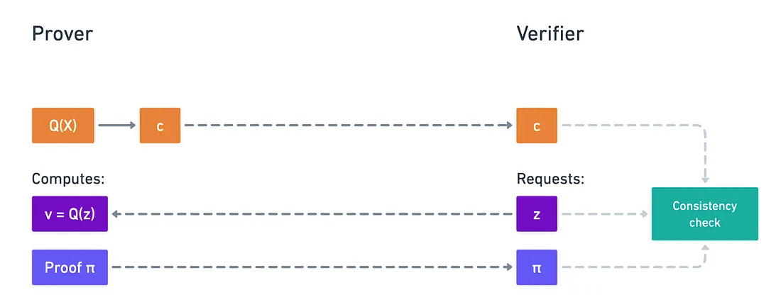
Naturally, we need to figure out how to build the proof $\pi$. And this is where things get a little more tricky.

Before we even get to use pairings at all, we first need to construct what’s called a witness polynomial. It’s a neat little trick, but it needs special attention since it’s a crucial piece in the success of KZG.

What we do is essentially transform the assertion $v = Q(z)$ into something that can actually be checked. For this, we define the polynomial $H(X)$ as:

$$H(X) = Q(X) {-} v$$

At surface level, this looks fairly inconsequential. However, we know something about this polynomial that we can use to our advantage: it has a root at $X = z$.

As long as the prover is honest and actually $v = Q(z)$ holds!

If there’s one thing we know about roots, it’s that we can rewrite the polynomial as:

$$H(X) = Q(X) {-} v = W(X)(X-z)$$

That $W(X)$ right there is the quotient polynomial of $H(X)$ and $(X {-} z)$. In other words, $(X {-} z)$ perfectly divides $H(X)$, leaving no remainder:

$$W(X) = \frac{Q(X) {-} v}{X {-} z}$$

And, again, this is only true so long as the evaluation $v = Q(z)$ is correct. 

Perfect! That’s all we need, really, because the proof $\pi$ is computed from this witness polynomial, and it’s simply:

$$\pi = g^{W(\tau)}$$

Where we use the SRS to calculate this once more.

Yeah, I know it’s a bit confusing  -  but we haven’t even gotten to the crazier part. Because now, the verifier has to check that proof using the original commitment $c$. This is the part where pairings are needed.

We’ll require a self-pairing between groups $\mathbb{G}$ and $\mathbb{G}_t$, and with it, the verifier will check this equality here:

$$e(c \cdot g^{-v}, g) \overset{?}{=} e(\pi, g^{\tau} \cdot g^{-z})$$

I know, it’s pretty mind-bending! I suggest taking a breather to fully wrap your head around this. In fact, I invite you to try and check that expression for correctness  - it’s a fun little exercise to grasp how bilinearity works. At its core, what this is doing is checking that the commitment and the proof are consistent, using that witness polynomial relation and bilinearity to tie everything together.

Showing that it’s binding is a little more involved, but the core idea is that producing a valid proof $\pi$ for an incorrect $v$ happens to be equivalent to solving a variant of the DDH problem we discussed earlier, that happens to still be hard even for pairing-friendly groups!

And that’s KZG in all of its glory!

Breaking the Scheme

Before we close the chapter on this method though, I want to show you exactly how easy it is to break it with knowledge of the secret $\tau$, so we can fully gauge the importance of discarding it.

Suppose for a second $\tau$ is known. The verifier asks for some opening $Q(z)$, and even though the correct evaluation is $v = Q(z)$, we’d like to convince them that the result is actually some other value $y$. What do we need to do to achieve this?

What we need is to forge a proof $\pi'$ so that it passes validation. That’s all! So let’s work backwards from there.

The check being performed relies on the expected structure of the witness polynomial: it’s possible to divide $Q(X) {-} v$ because we know there’s a root at $X = z$. This gives us a set of coefficients that we can use to calculate $\pi$ using the SRS, because that’s the only way to get $\pi$ without knowing $\tau$.

If we try to calculate a witness polynomial for the false value $y$, we’d run into a problem, because $y$ is not a root of our original $H(X)$, and thus we’d have a remainder when dividing by $(X {-} z)$. And so, this expression right here would not be a polynomial, but just a rational function:

$$W’(X) = \frac{Q(X) {-} y}{X {-} z}$$

But... if we know $\tau$, then who cares? You can just calculate $W'(\tau)$ directly! And the false proof would just be:

$$\pi‘ = g^{W’(\tau)}$$

Only this time, we are able to calculate it directly.

That’s it. It doesn’t take much to produce that forged proof. Hence the need to get rid of the secret value. It truly is toxic waste.

Phew! That was a lot!

We could analyze this further, but I think that’s enough for us here.

My brain is fried after writing this, and I can imagine you guys are on the same boat while reading!

What’s neat about KZG is that both the commitment and the proof are a single group element. That’s very lean, and ideal to keep some upcoming protocols inexpensive. It’s a nice selling point  - but it’s only as good as our ability to keep that secret value $\tau$ undisclosed.

Summary

And with that, we have our first fully functional polynomial commitment scheme!

This means we have at least one way to go about those oracle queries we talked about in previous encounters. Not only does this complete our description of the sum-check protocol from what feels like ages ago, but also it enables a whole new world of possibilities.

Sure, KZG is not the only possible solution (we already mentioned FRI, but we’ll also explore other options), and research continues to come up with new and improved PCSs that can make verifiable computing even more efficient.

Although, I must say, KZG is a very elegant solution already, and especially lean in terms of communication: both the commitment to the polynomial and the proof of correctness are a single group element. That’s going to matter a lot when we start plugging it into full proving systems!

And crucially, we introduced an important piece of math that can be really useful: pairings!

Perhaps the most questionable aspect of KZG is its trusted setup. I’ve been pretty adamant about it, because we know the possibility for safer setups exists.

Even though there are tradeoffs, it’s a direction we definitely need to explore.

To get us there, I want us to explore a whole family of knowledge arguments next, which comprise an important set of ideas that are absolutely a must-have in our quest for zero knowledge.

So I’ll see you on the next one!